Antigen presentation and tumor immunogenicity in cancer immunotherapy response prediction
Antigen presentation and tumor immunogenicity in cancer immunotherapy response prediction
- Dependencies
- Data download and preprocessing
- TCGA Pan-cancer data download
- TCGA pan-cancer data clean
- Selection of APM genes and marker genes of immune cell type
- Calculation of APS, TIS and IIS
- TIMER data download and clean
- TCGA mutation download and clean
- GEO datasets download and processing
- Immunotherapy clinical studies and genomics datasets
- TCGA Pan-cancer analyses
- Immunotherapy datasets analyses
- Supplementary analyses
Please note this work under Apache License v2 license, copyright belongs to Shixiang Wang and Xue-Song Liu. And the study has been applied for a national patent in China.
This document is compiled from an Rmarkdown file which contains all code or description necessary to reproduce the analysis for the accompanying project. Each section below describes a different component of the analysis and all numbers and figures are generated directly from the underlying data on compilation.
Dependencies
The preprocessing step is dependent on R software and some R packages, if you have not used R yet or R is not installed, please see https://cran.r-project.org/.
R packages:
- UCSCXenaTools - download data from UCSC Xena
- GEOquery - download data from NCBI GEO database
- tidyverse - operate data, plot
- data.table - operate data
- survival - built in R, used to do survival analysis
- metafor, metawho - meta-analysis
- forestmodel - generate forestplot for meta-analysis model
- forestplot - plot forestplot
- survminer - plot survival fit
- pROC - ROC analysis and visualization
- TCGAmutations - download TCGA mutation data
- DT - show data table as a table in html
- GSVA - GSVA algorithm implementation
- ggstatsplot - plot scatter with linear fit
- corrplot - plot correlation
- knitr, rmdformats - used to compile this file
- readxl - read xlsx data
- Some other dependent packages
These R packages are easily searched by internet and installed from either CRAN or Bioconductor, they have no strict version requirements to reproduce the following analyses.
Data download and preprocessing
This part will clearly describe how to process raw data but not provide an easy script for re-running all preprocess steps just by a click due to the complexity of data preprocessing.
TCGA Pan-cancer data download
TCGA Pan-cancer data (Version 2017-10-13), including datasets of clinical informaiton, gene expression, are downloaded from UCSC Xena via R package UCSCXenaTools.
UCSCXenaTools is developed by Shixiang and it is an R package to robustly access data from UCSC Xena data hubs. More please see paper: Wang et al., (2019). The UCSCXenaTools R package: a toolkit for accessing genomics data from UCSC Xena platform, from cancer multi-omics to single-cell RNA-seq. Journal of Open Source Software, 4(40), 1627, https://doi.org/10.21105/joss.01627
If you have not installed this package yet, please run following command in R.
Load the package with:
Obtain datasets information available at TCGA data hubs of UCSC Xena:
xe <- XenaGenerate(subset = XenaHostNames == "tcgaHub")
xe
#> class: XenaHub
#> hosts():
#>   https://tcga.xenahubs.net
#> cohorts() (38 total):
#>   TCGA Ovarian Cancer (OV)
#>   TCGA Kidney Clear Cell Carcinoma (KIRC)
#>   TCGA Lower Grade Glioma (LGG)
#>   ...
#>   TCGA Colon Cancer (COAD)
#>   TCGA Formalin Fixed Paraffin-Embedded Pilot Phase II (FPPP)
#> datasets() (879 total):
#>   TCGA.OV.sampleMap/HumanMethylation27
#>   TCGA.OV.sampleMap/HumanMethylation450
#>   TCGA.OV.sampleMap/Gistic2_CopyNumber_Gistic2_all_data_by_genes
#>   ...
#>   TCGA.FPPP.sampleMap/miRNA_HiSeq_gene
#>   TCGA.FPPP.sampleMap/FPPP_clinicalMatrix
Obtain clinical datasets of TCGA:
xe %>% XenaFilter(filterDatasets = "clinical") -> xe_clinical
xe_clinical
#> class: XenaHub
#> hosts():
#>   https://tcga.xenahubs.net
#> cohorts() (37 total):
#>   TCGA Ovarian Cancer (OV)
#>   TCGA Kidney Clear Cell Carcinoma (KIRC)
#>   TCGA Lower Grade Glioma (LGG)
#>   ...
#>   TCGA Colon Cancer (COAD)
#>   TCGA Formalin Fixed Paraffin-Embedded Pilot Phase II (FPPP)
#> datasets() (37 total):
#>   TCGA.OV.sampleMap/OV_clinicalMatrix
#>   TCGA.KIRC.sampleMap/KIRC_clinicalMatrix
#>   TCGA.LGG.sampleMap/LGG_clinicalMatrix
#>   ...
#>   TCGA.COAD.sampleMap/COAD_clinicalMatrix
#>   TCGA.FPPP.sampleMap/FPPP_clinicalMatrix
Obtain gene expression datasets of TCGA:
xe %>% XenaFilter(filterDatasets = "HiSeqV2_PANCAN$") -> xe_rna_pancan
xe_rna_pancan
#> class: XenaHub
#> hosts():
#>   https://tcga.xenahubs.net
#> cohorts() (36 total):
#>   TCGA Ovarian Cancer (OV)
#>   TCGA Kidney Clear Cell Carcinoma (KIRC)
#>   TCGA Lower Grade Glioma (LGG)
#>   ...
#>   TCGA Uterine Carcinosarcoma (UCS)
#>   TCGA Colon Cancer (COAD)
#> datasets() (36 total):
#>   TCGA.OV.sampleMap/HiSeqV2_PANCAN
#>   TCGA.KIRC.sampleMap/HiSeqV2_PANCAN
#>   TCGA.LGG.sampleMap/HiSeqV2_PANCAN
#>   ...
#>   TCGA.UCS.sampleMap/HiSeqV2_PANCAN
#>   TCGA.COAD.sampleMap/HiSeqV2_PANCAN
Create data queries and download them:
xe_clinical.query <- XenaQuery(xe_clinical)
xe_clinical.download <- XenaDownload(xe_clinical.query,
  destdir = "UCSC_Xena/TCGA/Clinical", trans_slash = TRUE, force = TRUE
)

xe_rna_pancan.query <- XenaQuery(xe_rna_pancan)
xe_rna_pancan.download <- XenaDownload(xe_rna_pancan.query,
  destdir = "UCSC_Xena/TCGA/RNAseq_Pancan", trans_slash = TRUE
)
The RNASeq data we downloaded are pancan normalized.
For comparing data within independent cohort (like TCGA-LUAD), we recommend to use the “gene expression RNAseq” dataset. For questions regarding the gene expression of this particular cohort in relation to other types tumors, you can use the pancan normalized version of the “gene expression RNAseq” data. For comparing with data outside TCGA, we recommend using the percentile version if the non-TCGA data is normalized by percentile ranking. For more information, please see our Data FAQ: here.
These datasets are downloaded to local machine, we need to load them into R. However, whether filenames of datasets or contents in datasets all look messy, next we need to clean them before real analysis.
TCGA pan-cancer data clean
Clean filenames
First, clean filenames.
# set data directory where TCGA clinical and pancan RNAseq data stored
TCGA_DIR <- "UCSC_Xena/TCGA"
# obtain filenames of rna-seq data
dir(paste0(TCGA_DIR, "/RNAseq_Pancan")) -> RNAseq_filelist
# obtain tcga project code
sub("TCGA\\.(.*)\\.sampleMap.*", "\\1", RNAseq_filelist) -> project_code
# obtain filenames of clinical datasets
dir(paste0(TCGA_DIR, "/Clinical")) -> Clinical_filelist
Check.
head(RNAseq_filelist)
#> [1] "TCGA.ACC.sampleMap__HiSeqV2_PANCAN.gz"
#> [2] "TCGA.BLCA.sampleMap__HiSeqV2_PANCAN.gz"
#> [3] "TCGA.BRCA.sampleMap__HiSeqV2_PANCAN.gz"
#> [4] "TCGA.CESC.sampleMap__HiSeqV2_PANCAN.gz"
#> [5] "TCGA.CHOL.sampleMap__HiSeqV2_PANCAN.gz"
#> [6] "TCGA.COAD.sampleMap__HiSeqV2_PANCAN.gz"

head(project_code)
#> [1] "ACC"  "BLCA" "BRCA" "CESC" "CHOL" "COAD"

head(Clinical_filelist)
#> [1] "TCGA.ACC.sampleMap__ACC_clinicalMatrix.gz"
#> [2] "TCGA.BLCA.sampleMap__BLCA_clinicalMatrix.gz"
#> [3] "TCGA.BRCA.sampleMap__BRCA_clinicalMatrix.gz"
#> [4] "TCGA.CESC.sampleMap__CESC_clinicalMatrix.gz"
#> [5] "TCGA.CHOL.sampleMap__CHOL_clinicalMatrix.gz"
#> [6] "TCGA.COAD.sampleMap__COAD_clinicalMatrix.gz"
Obtain TCGA project abbreviations from https://gdc.cancer.gov/resources-tcga-users/tcga-code-tables/tcga-study-abbreviations and read as a data.frame in R.
library(readr)
TCGA_Study <- read_tsv("
                      LAML  Acute Myeloid Leukemia
                      ACC   Adrenocortical carcinoma
                      BLCA  Bladder Urothelial Carcinoma
                      LGG   Brain Lower Grade Glioma
                      BRCA  Breast invasive carcinoma
                      CESC  Cervical squamous cell carcinoma and endocervical adenocarcinoma
                      CHOL  Cholangiocarcinoma
                      LCML  Chronic Myelogenous Leukemia
                      COAD  Colon adenocarcinoma
                      CNTL  Controls
                      ESCA  Esophageal carcinoma
                      FPPP  FFPE Pilot Phase II
                      GBM   Glioblastoma multiforme
                      HNSC  Head and Neck squamous cell carcinoma
                      KICH  Kidney Chromophobe
                      KIRC  Kidney renal clear cell carcinoma
                      KIRP  Kidney renal papillary cell carcinoma
                      LIHC  Liver hepatocellular carcinoma
                      LUAD  Lung adenocarcinoma
                      LUSC  Lung squamous cell carcinoma
                      DLBC  Lymphoid Neoplasm Diffuse Large B-cell Lymphoma
                      MESO  Mesothelioma
                      MISC  Miscellaneous
                      OV    Ovarian serous cystadenocarcinoma
                      PAAD  Pancreatic adenocarcinoma
                      PCPG  Pheochromocytoma and Paraganglioma
                      PRAD  Prostate adenocarcinoma
                      READ  Rectum adenocarcinoma
                      SARC  Sarcoma
                      SKCM  Skin Cutaneous Melanoma
                      STAD  Stomach adenocarcinoma
                      TGCT  Testicular Germ Cell Tumors
                      THYM  Thymoma
                      THCA  Thyroid carcinoma
                      UCS   Uterine Carcinosarcoma
                      UCEC  Uterine Corpus Endometrial Carcinoma
                      UVM   Uveal Melanoma", col_names = FALSE)
colnames(TCGA_Study) <- c("StudyAbbreviation", "StudyName")
Compare difference.
intersect(project_code, TCGA_Study$StudyAbbreviation) -> project_code
Clinical_filelist[rowSums(sapply(paste0("__", project_code, "_"), function(x) grepl(x, Clinical_filelist))) > 0] -> Clinical_filelist2

setdiff(Clinical_filelist, Clinical_filelist2)
#> [1] "TCGA.COADREAD.sampleMap__COADREAD_clinicalMatrix.gz"
#> [2] "TCGA.FPPP.sampleMap__FPPP_clinicalMatrix.gz"
#> [3] "TCGA.GBMLGG.sampleMap__GBMLGG_clinicalMatrix.gz"
#> [4] "TCGA.LUNG.sampleMap__LUNG_clinicalMatrix.gz"
Remove TCGA.FPPP.sampleMap__FPPP_clinicalMatrix.gz which has no RNAseq data. Remove other 3 datasets which merge more than one TCGA study, only keep individual study from TCGA.
Clean clinical datasets
Now, we read TCGA clinical datasets and clean them.
library(tidyverse)
#> ── Attaching packages ─────────────────────────────────────────────────────────────────── tidyverse 1.2.1 ──
#> ✔ ggplot2 3.2.1     ✔ purrr   0.3.3
#> ✔ tibble  2.1.3     ✔ stringr 1.4.0
#> ✔ tidyr   1.0.0     ✔ forcats 0.4.0
#> ── Conflicts ────────────────────────────────────────────────────────────────────── tidyverse_conflicts() ──
#> ✖ dplyr::filter() masks stats::filter()
#> ✖ dplyr::lag()    masks stats::lag()
# keep valuable columns of clinical datasets
select_cols <- c(
  "sampleID", "OS", "OS.time", "OS.unit", "RFS", "RFS.time", "RFS.unit",
  "age_at_initial_pathologic_diagnosis", "gender", "tobacco_smoking_history",
  "tobacco_smoking_history_indicator", "sample_type", "pathologic_M",
  "pathologic_N", "pathologic_T", "pathologic_stage"
)

# read clinical files
Cli_DIR <- paste0(TCGA_DIR, "/Clinical")

#----------------------------------
# Load and preprocess clinical data
#----------------------------------
Clinical_List <- XenaPrepare(paste0(Cli_DIR, "/", Clinical_filelist2))
names(Clinical_List)
#>  [1] "TCGA.ACC.sampleMap__ACC_clinicalMatrix.gz"
#>  [2] "TCGA.BLCA.sampleMap__BLCA_clinicalMatrix.gz"
#>  [3] "TCGA.BRCA.sampleMap__BRCA_clinicalMatrix.gz"
#>  [4] "TCGA.CESC.sampleMap__CESC_clinicalMatrix.gz"
#>  [5] "TCGA.CHOL.sampleMap__CHOL_clinicalMatrix.gz"
#>  [6] "TCGA.COAD.sampleMap__COAD_clinicalMatrix.gz"
#>  [7] "TCGA.DLBC.sampleMap__DLBC_clinicalMatrix.gz"
#>  [8] "TCGA.ESCA.sampleMap__ESCA_clinicalMatrix.gz"
#>  [9] "TCGA.GBM.sampleMap__GBM_clinicalMatrix.gz"
#> [10] "TCGA.HNSC.sampleMap__HNSC_clinicalMatrix.gz"
#> [11] "TCGA.KICH.sampleMap__KICH_clinicalMatrix.gz"
#> [12] "TCGA.KIRC.sampleMap__KIRC_clinicalMatrix.gz"
#> [13] "TCGA.KIRP.sampleMap__KIRP_clinicalMatrix.gz"
#> [14] "TCGA.LAML.sampleMap__LAML_clinicalMatrix.gz"
#> [15] "TCGA.LGG.sampleMap__LGG_clinicalMatrix.gz"
#> [16] "TCGA.LIHC.sampleMap__LIHC_clinicalMatrix.gz"
#> [17] "TCGA.LUAD.sampleMap__LUAD_clinicalMatrix.gz"
#> [18] "TCGA.LUSC.sampleMap__LUSC_clinicalMatrix.gz"
#> [19] "TCGA.MESO.sampleMap__MESO_clinicalMatrix.gz"
#> [20] "TCGA.OV.sampleMap__OV_clinicalMatrix.gz"
#> [21] "TCGA.PAAD.sampleMap__PAAD_clinicalMatrix.gz"
#> [22] "TCGA.PCPG.sampleMap__PCPG_clinicalMatrix.gz"
#> [23] "TCGA.PRAD.sampleMap__PRAD_clinicalMatrix.gz"
#> [24] "TCGA.READ.sampleMap__READ_clinicalMatrix.gz"
#> [25] "TCGA.SARC.sampleMap__SARC_clinicalMatrix.gz"
#> [26] "TCGA.SKCM.sampleMap__SKCM_clinicalMatrix.gz"
#> [27] "TCGA.STAD.sampleMap__STAD_clinicalMatrix.gz"
#> [28] "TCGA.TGCT.sampleMap__TGCT_clinicalMatrix.gz"
#> [29] "TCGA.THCA.sampleMap__THCA_clinicalMatrix.gz"
#> [30] "TCGA.THYM.sampleMap__THYM_clinicalMatrix.gz"
#> [31] "TCGA.UCEC.sampleMap__UCEC_clinicalMatrix.gz"
#> [32] "TCGA.UCS.sampleMap__UCS_clinicalMatrix.gz"
#> [33] "TCGA.UVM.sampleMap__UVM_clinicalMatrix.gz"
sub("TCGA\\.(.*)\\.sampleMap.*", "\\1", names(Clinical_List)) -> project_code

TCGA_Clinical <- tibble()
# for loop
for (i in 1:length(project_code)) {
  clinical <- names(Clinical_List)[i]
  project <- project_code[i]
  df <- Clinical_List[[clinical]]
  col_exist <- select_cols %in% colnames(df)
  res <- tibble()
  if (!all(col_exist)) {
    res <- df[, select_cols[col_exist]]
    res[, select_cols[!col_exist]] <- NA
  } else {
    res <- df[, select_cols]
  }
  res$Project <- project
  res %>% select(Project, select_cols) -> res
  TCGA_Clinical <- bind_rows(TCGA_Clinical, res)
}

rm(res, df, i, clinical, project, col_exist) # remove temp variables
View the clinical data, check variables.
All unit are same in days, remove two column with redundant information.
Continue to tidy clinical datasets: rename variables, filter 14 samples with unusual sample types, rename variable value and . After cleanning, save the result object TCGA_Clinical.tidy for following analysis.
# create a new tidy dataframe
TCGA_Clinical.tidy <- TCGA_Clinical %>%
  rename(
    Age = age_at_initial_pathologic_diagnosis, Gender = gender,
    Smoking_history = tobacco_smoking_history,
    Smoking_indicator = tobacco_smoking_history_indicator,
    Tumor_Sample_Barcode = sampleID
  ) %>%
  filter(sample_type %in% c(
    "Solid Tissue Normal", "Primary Tumor", "Metastatic", "Recurrent Tumor",
    "Primary Blood Derived Cancer - Peripheral Blood"
  )) %>% # Additional - New Primary, Additional Metastatic, FFPE Scrolls total 14 sample removed
  mutate(Gender = case_when(
    Gender == "FEMALE" ~ "Female",
    Gender == "MALE" ~ "Male",
    TRUE ~ NA_character_
  ), Tumor_stage = case_when(
    pathologic_stage == "Stage 0" ~ "0",
    pathologic_stage %in% c("Stage I", "Stage IA", "Stage IB") ~ "I",
    pathologic_stage %in% c("Stage II", "Stage IIA", "Stage IIB", "Stage IIC") ~ "II",
    pathologic_stage %in% c("Stage IIIA", "Stage IIIB", "Stage IIIC") ~ "III",
    pathologic_stage %in% c("Stage IV", "Stage IVA", "Stage IVB", "Stage IVC") ~ "IV",
    pathologic_stage == "Stage X" ~ "X",
    TRUE ~ NA_character_
  )) %>%
  mutate(
    Gender = factor(Gender, levels = c("Male", "Female")),
    Tumor_stage = factor(Tumor_stage, levels = c("0", "I", "II", "III", "IV", "X"))
  )

if (!file.exists("results/TCGA_tidy_Clinical.RData")) {
  dir.create("results", showWarnings = FALSE)
  save(TCGA_Clinical.tidy, file = "results/TCGA_tidy_Clinical.RData")
}
Clean RNASeq datasets
Now, we read TCGA pan-cancer RNASeq datasets and clean them.
dir(paste0(TCGA_DIR, "/RNAseq_Pancan")) -> RNAseq_filelist.Pancan
RNAseq_filelist.Pancan[rowSums(sapply(paste0("TCGA.", project_code, ".sampleMap"), function(x) grepl(x, RNAseq_filelist.Pancan))) > 0] -> RNAseq_filelist.Pancan2

RNASeqDIR.pancan <- paste0(TCGA_DIR, "/RNAseq_Pancan")
RNASeq_List.pancan <- XenaPrepare(paste0(RNASeqDIR.pancan, "/", RNAseq_filelist.Pancan2))
names(RNASeq_List.pancan)
sapply(RNASeq_List.pancan, function(x) nrow(x))

names(RNASeq_List.pancan) <- sub("TCGA\\.(.*)\\.sampleMap.*", "\\1", names(RNASeq_List.pancan))

RNASeq_pancan <- purrr::reduce(RNASeq_List.pancan, full_join)
if (!file.exists("results/TCGA_RNASeq_PanCancer.RData")) {
  save(RNASeq_pancan, file = "results/TCGA_RNASeq_PanCancer.RData")
}


# class(RNASeq_pancan)
rm(RNASeq_List.pancan)
The result object RNASeq_pancan is very huge, it needs about 1.5GB space to store. We will not view it as a table in html page.
Selection of APM genes and marker genes of immune cell type
Marker genes for immune cell types were obtained from Senbabaoglu, Y. et al, selection of genes involved in processing and presentation of antigen (APM) was also inspired by this paper and finally 18 genes were selected based on literature review of APM and some facts that mutations or deletions affecting genes encoding APM (HLA, beta2-microglobulin, TAP1/2 etc.) may lead to reduced presentation of neoantigens by a cancer cell.
APM_genes <- read_csv("../data/APM.csv", skip = 1)

immune_cellType <- read_csv("../data/Immune_Cell_type_List.csv", skip = 1)
immune_cellType <- immune_cellType %>% filter(inRNAseq == "YES")

# merge two gene list
merged_geneList <- bind_rows(
  immune_cellType,
  tibble(
    Cell_type = "APM", Symbol = APM_genes$Gene_Name,
    Name = APM_genes$Protein_Name, inRNAseq = "YES"
  )
)

# save data
if (!file.exists("results/merged_geneList.RData")) {
  save(merged_geneList, file = "results/merged_geneList.RData")
}
View gene list.
Remove all variables.
Calculation of APS, TIS and IIS
The GSVA package allows one to perform a change in coordinate systems of molecular measurements, transforming the data from a gene by sample matrix to a gene-set by sample matrix, thereby allowing the evaluation of pathway enrichment for each sample. This new matrix of GSVA enrichment scores facilitates applying standard analytical methods like functional enrichment, survival analysis, clustering, CNV-pathway analysis or cross-tissue pathway analysis, in a pathway-centric manner.
APM score (APS) and score of each immune cell type are directly calculated from GSVA method. Aggregate TIS (T cell infiltration score) and IIS (Immune cell infiltration score) are calculated using following method, their effectiveness have been validated by many studies.
The TIS was defined as the mean of the standardized values for the following T cell subsets: CD8 T, T helper, T, T central and effector memory, Th1, Th2, Th17, and Treg cells. The immune infiltration score (IIS) for a sample was defined as the mean of standardized values for macrophages, DC subsets (total, plasmacytoid, immature, activated), B cells, cytotoxic cells, eosinophils, mast cells, neutrophils, NK cell subsets (total, CD56 bright, CD56 dim), and all T cell subsets (CD8 T, T helper, T central and effector memory, Th1, Th2, Th17, and Treg cells). (Senbabaoglu, Y. et al)
Load function used to apply GSVA method.
Apply GSVA to TCGA data. This step should run on a machine with big memory.
# load data
load("results/merged_geneList.RData")
load("results/TCGA_RNASeq_PanCancer.RData")


applyGSVA(merged_geneList, group_col = "Cell_type", gene_col = "Symbol", ExprMatList = list(RNASeq_pancan), method = "gsva") -> res_pancan.GSVA

save(res_pancan.GSVA, file = "results/res_pancan.GSVA.RData")
Calculate TIS and IIS.
if (!exists("res_pancan.GSVA")) {
  load("results/res_pancan.GSVA.RData")
}

res_pancan.GSVA <- res_pancan.GSVA[[1]]

calc_TisIIs <- function(df) {
  df %>%
    mutate(
      TIS = (`CD8 T cells` + `T helper cells` + `T cells` + `Tcm cells` + `Tem cells` + `Th1 cells` + `Th2 cells` + `Th17 cells` + `Treg cells`) / 9,
      IIS = (`CD8 T cells` + `T helper cells` + `T cells` + `Tcm cells` + `Tem cells` + `Th1 cells` + `Th2 cells` + `Th17 cells` + `Treg cells` + aDC + `B cells` + `Cytotoxic cells` + DC + Eosinophils + iDC + Macrophages + `Mast cells` + Neutrophils + `NK CD56bright cells` + `NK CD56dim cells` + `NK cells` + pDC) / 22
    ) -> df
}

# tidy res_pancan.GSVA
res_pancan.GSVA <- rownames_to_column(res_pancan.GSVA, var = "tsb")

# calculate TIS and IIS
gsva.pac <- calc_TisIIs(res_pancan.GSVA)
View this table (head 100 rows).
save GSVA scores of APM and immune cell types, TIS and IIS.
if (!file.exists("results/gsva_tcga_pancan.RData")) {
  save(gsva.pac, file = "results/gsva_tcga_pancan.RData")
}

rm(list = ls())
Calculation of APS7
Here we update a new analysis about calculating APS based on 7 APM gene signature from Senbabaoglu, Y. et al. We name this score as ‘APS7’.
TIMER data download and clean
TIMER is a method that can accurately resolve relative fractions of diverse cell types based on gene expression profiles from complex tissues. We downloaded TIMER result for TCGA samples from Li, B. et al..
Load TIMER result and clean it for use.
timer <- read_tsv("../data/TCGA_sixcell_population_TIMER.txt")
timer$sample %>% length()
#> [1] 10009
timer$sample %>%
  unique() %>%
  length()
#> [1] 9990
timer$sample %>%
  substr(start = 1, stop = 12) %>%
  unique() %>%
  length()
#> [1] 9262

# keep only tumor samples
timer %>%
  filter(as.numeric(substr(sample, 14, 15)) %in% seq(1, 9)) %>%
  mutate(sample = substr(sample, 1, 15)) -> timer_clean
timer_clean %>%
  arrange(desc(T_cell.CD8)) %>%
  distinct(sample, .keep_all = TRUE) -> timer_clean

# save
if (!file.exists("results/timer.RData")) {
  save(timer_clean, file = "results/timer.RData")
}

rm(list = ls())
TCGA mutation download and clean
We downloaded TCGA somatic mutations (data source: TCGA MC3) via TCGAmutations package.
TCGAmutations is an R data package containing somatic mutations from TCGA cohorts. This is particularly useful for those working with mutation data from TCGA studies - where most of the time is spent on searching various databases, downloading, compiling and tidying up the data before even the actual analysis is started. This package tries to mitigate the issue by providing pre-compiled, curated somatic mutations from 33 TCGA cohorts along with relevant clinical information for all sequenced samples.
Load mutations of TCGA studies and merge them into one.
## install package please use following command
# devtools::install_github(repo = "PoisonAlien/TCGAmutations")

# load package
require(TCGAmutations)


study_list <- tcga_available()$Study_Abbreviation[-34]
cohorts <- system.file("extdata", "cohorts.txt", package = "TCGAmutations")
cohorts <- data.table::fread(input = cohorts)

# calculate TMB
lapply(study_list, function(study) {
  require(maftools)
  TCGAmutations::tcga_load(study)
  maf <- eval(as.symbol(tolower(paste0("TCGA_", study, "_mc3"))))
  maf.silent <- maf@maf.silent
  sample.silent <- maf.silent[, .N, .(Tumor_Sample_Barcode)]
  sample.nonsilent <- getSampleSummary(maf)
  res <- dplyr::full_join(sample.silent, sample.nonsilent, by = "Tumor_Sample_Barcode")
  res <- res %>%
    dplyr::mutate(
      TMB_Total = ifelse(!is.na(N), N + total, total),
      TMB_NonsynSNP = Missense_Mutation + Nonsense_Mutation,
      TMB_NonsynVariants = total
    ) %>%
    dplyr::select(TMB_Total:TMB_NonsynVariants, Tumor_Sample_Barcode)
  res
}) -> tcga_tmb
names(tcga_tmb) <- study_list

# 33 study available, merge them
TCGA_TMB <- purrr::reduce(tcga_tmb, bind_rows)

if (!file.exists("results/TCGA_TMB.RData")) {
  save(TCGA_TMB, file = "results/TCGA_TMB.RData")
}

# rm(list = grep("tcga_*", ls(), value = TRUE))
rm(list = ls())
GEO datasets download and processing
We also tried our best to collect gene expression data to extend APM score (APS), IIS etc. calculation for more cancer types by searching NCBI GEO databases. We only focus on looking for cancer types which showed in list of our immunotherapy clinical studies and not showed in TCGA studies. Finally, we found 5 GEO datasets which can extract gene expression data of Merkel Cell Carcinoma, Small Cell Lung Cancer and Cutaneous Squamous Carcinoma. Download of these datasets need R package GEOquery is installed. Following code showed how we downloaded and carefully processed them.
#----------------------------------------------------------------
# Purpose:
# Add APM data from GEO for some tumor types
# Include Merkel Cell Carcinoma and Small Cell Lung Cancer
#         and Cutaneous Squamous Carcinoma
#----------------------------------------------------------------
library(GEOquery)
library(tidyverse)

if (!dir.exists("../data/GEOdata")) {
  dir.create("../data/GEOdata")
}

geo_dir <- "../data/GEOdata"

GSE_39612 <- getGEO("GSE39612", GSEMatrix = TRUE, AnnotGPL = TRUE, destdir = geo_dir)
GSE_22396 <- getGEO("GSE22396", GSEMatrix = TRUE, AnnotGPL = TRUE, destdir = geo_dir)
GSE_36150 <- getGEO("GSE36150", GSEMatrix = TRUE, AnnotGPL = TRUE, destdir = geo_dir)
GSE_50451 <- getGEO("GSE50451", GSEMatrix = TRUE, AnnotGPL = TRUE, destdir = geo_dir)
GSE_99316 <- getGEO("GSE99316", GSEMatrix = TRUE, AnnotGPL = TRUE, destdir = geo_dir)

exprs(GSE_22396$GSE22396_series_matrix.txt.gz) %>% nrow()
pData(GSE_22396$GSE22396_series_matrix.txt.gz)
fData(GSE_22396$GSE22396_series_matrix.txt.gz) %>% nrow()

#---------------------------------------------------------
# process GSE_39612
gset1 <- GSE_39612$GSE39612_series_matrix.txt.gz
View(pData(gset1))

gset1_mcc <- gset1[, grep("MCC", gset1$title)]
gset1_scc <- gset1[, grep("SCC", gset1$title)]

rm(gset1)
# process GSE_22396
gset2 <- GSE_22396$GSE22396_series_matrix.txt.gz
View(pData(gset2))

# process GSE_36150
gset3 <- GSE_36150$GSE36150_series_matrix.txt.gz
View(pData(gset3))

# process GSE_50451
gset4_1 <- GSE_50451$`GSE50451-GPL570_series_matrix.txt.gz`
gset4_2 <- GSE_50451$`GSE50451-GPL571_series_matrix.txt.gz`

View(pData(gset4_1))
View(pData(gset4_2))
# gset4_1 all cell_lines, not use it
#
gset4_mcc <- gset4_2[, grep("MCC tumor", gset4_2$source_name_ch1)]
gset4_sclc <- gset4_2[, grep("SCLC tumor", gset4_2$source_name_ch1)]

rm(gset4_1, gset4_2)
# process GSE_99316
gset5_1 <- GSE_99316$`GSE99316-GPL10999_series_matrix.txt.gz`
gset5_2 <- GSE_99316$`GSE99316-GPL570_series_matrix.txt.gz`
gset5_3 <- GSE_99316$`GSE99316-GPL96_series_matrix.txt.gz`
gset5_4 <- GSE_99316$`GSE99316-GPL97_series_matrix.txt.gz`

View(pData(gset5_1))
View(pData(gset5_2))
View(pData(gset5_3))
View(pData(gset5_4))

# only gset5_2 has data we need
gset5_sclc <- gset5_2[, grep("SCLC", gset5_2$title)]

rm(gset5_1, gset5_2, gset5_3, gset5_4)

#-------------------------------------------------
# Now summary data
merkel_data <- list(gset1_mcc, gset2, gset3, gset4_mcc)
scc_data <- list(gset1_scc)
sclc_data <- list(gset4_sclc, gset5_sclc)

#--------------------
# apply GSVA method
load("results/merged_geneList.RData")

# transform exprset to tibble
genTibbleList <- function(gsetList) {
  stopifnot(is.list(gsetList), require("Biobase"), require("tidyverse"), class(gsetList[[1]]) == "ExpressionSet")

  res <- list()
  i <- 1
  for (gset in gsetList) {
    eset <- exprs(gset)
    # find gene symbol column
    fdata <- fData(gset)
    symbol_col <- grep("^gene.?symbol", colnames(fdata), value = TRUE, ignore.case = TRUE)

    if (length(symbol_col) == 0) {
      message("Find nothing about gene symbol in fData, try search it...")
      symbol_col2 <- grep("^gene_assignment", colnames(fdata), value = TRUE, ignore.case = TRUE)
      message("find ", symbol_col2)

      message("processing...")
      strlist <- strsplit(fdata[, symbol_col2], split = " // ")
      rowname <- sapply(strlist, function(x) trimws(x[2]))
      rownames(eset) <- rowname

      # stop("Something wrong with your fData of input List, please check it")
    }
    if (length(symbol_col) > 1) {
      warning("Multiple columns of fData match gene symbol, only use the first one")
      symbol_col <- symbol_col[1]
      rownames(eset) <- fdata[, symbol_col]
    } else if (length(symbol_col) == 1){
      rownames(eset) <- fdata[, symbol_col]
    }

    # remove duplicate rows, keep the one with biggest mean value
    eset %>%
      as.data.frame() %>%
      rownames_to_column() %>%
      mutate(
        mean_expr = rowMeans(.[, -1], na.rm = TRUE),
        rowname = sub("^(\\w+)\\..*", "\\1", rowname)
      ) %>%
      arrange(rowname, desc(mean_expr)) %>%
      distinct(rowname, .keep_all = TRUE) %>%
      select(-mean_expr) %>%
      as.tibble() -> res[[i]]

    i <- i + 1
  }
  return(res)
}

# apply GSVA method
applyGSVA <- function(group_df, group_col, gene_col, ExprMatList,
                      method = c("ssgsea", "gsva", "zscore", "plage"),
                      kcdf = c("Gaussian", "Poisson")) {
  stopifnot(inherits(group_df, "tbl_df") &
    inherits(group_col, "character") &
    inherits(gene_col, "character") &
    inherits(ExprMatList, "list"))
  if (!require(GSVA)) {
    stop("GSVA package need to be installed!")
  }

  method <- match.arg(method)
  kcdf <- match.arg(kcdf)

  require(dplyr)

  i <- 1
  resList <- list()
  groups <- names(table(group_df[, group_col]))
  gset_list <- lapply(groups, function(x) {
    group_df[group_df[, group_col] == x, gene_col] %>%
      unlist() %>%
      as.character()
  })

  names(gset_list) <- groups

  for (expr_mat in ExprMatList) {
    if (!inherits(expr_mat, "tbl_df")) {
      stop("element of ExprMatList should be tibble!")
    }
    expr_mat <- as.data.frame(expr_mat)
    rownames(expr_mat) <- expr_mat[, 1]
    expr_mat <- expr_mat[, -1] %>% as.matrix()

    res <- gsva(expr = expr_mat, gset.idx.list = gset_list, method = method, kcdf = kcdf)
    res <- as.data.frame(t(res))
    colnames(res)[1] <- "tsb"
    resList[[i]] <- res
    names(resList)[i] <- names(ExprMatList)[i]
    i <- i + 1
  }
  return(resList)
}


## scc
tibble.scc <- genTibbleList(scc_data)
gsva.scc <- applyGSVA(merged_geneList,
  group_col = "Cell_type",
  gene_col = "Symbol", ExprMatList = tibble.scc, method = "gsva"
)
## sclc
tibble.sclc <- genTibbleList(sclc_data)
gsva.sclc <- applyGSVA(merged_geneList,
  group_col = "Cell_type",
  gene_col = "Symbol", ExprMatList = tibble.sclc, method = "gsva"
)

## merkel1
tibble.merkel <- genTibbleList(merkel_data)

gsva.merkel <- applyGSVA(merged_geneList,
  group_col = "Cell_type",
  gene_col = "Symbol", ExprMatList = tibble.merkel, method = "gsva"
)

save(gsva.scc, gsva.sclc, gsva.merkel, file = "results/Add_gsva_scc_sclc_merkel.RData")
Immunotherapy clinical studies and genomics datasets
Immunotherapy clinical studies
Collecting response rate of immunotherapy clinical studies was inspired by the paper Tumor Mutational Burden and Response Rate to PD-1 inhibition which published on journal NEJM, this paper showed data from about 50 stuides. However, detail values of response rate the authors collected were not published. We followed their search strategy and tried our best to find all clinical studies which recorded response rate. Totally, we reviewed abstract of over 100 clinical studies, collected response rate values, then carefully filtered them based on standard we set, selected the most respresenting data (from about 60 studies) for downstream analysis. More detail of this procedure please see Method section of our manuscript. The data we collected for analysi are double checked and open to readers as a supplementary table.
Immunotherapy genomics datasets
To evaluate the predictive power of TIGS in ICI clinical response prediction, we searched PubMed for ICI clinical studies with available individual patient’s TMB and gene transcriptome information. In total three datasets are identified after this search. Van Allen et al 2015 dataset was downloaded from supplementary files of reference. This dataset studied CTLA-4 blockade in metastatic melanoma, and “clinical benefit” was defined using a composite end point of complete response or partial response to CTLA-4 blockade by RECIST criteria or stable disease by RECIST criteria with overall survival greater than 1 year, “no clinical benefit” was defined as progressive disease by RECIST criteria or stable disease with overall survival less than 1 year. Hugo et al 2016 dataset was downloaded from supplementary files of reference. This dataset studied Anti-PD-1therapy in metastatic melanoma, responding tumors were derived from patients who have complete or partial responses or stable disease in response to anti-PD-1 therapy, non-responding tumors were derived from patients who had progressive disease. Snyder et al dataset was downloaded from https://github.com/hammerlab/multi-omic-urothelial-anti-pdl1. This dataset studied PD-L1 blockade in urothelial cancer, and durable clinical benefit was defined as progression-free survival >6 months. RNA-Seq data was used to calculate the APS for each patient. Only patients with both APS and TMB value were used to calculate the TIGS. Median of TMB or TIGS was used as the threshold to separate TMB High/Low group or TIGS High/Low group in Kaplan-Meier overall survival curve analysis.
Detail of how to process these 3 datasets will be described at analysis part.
TCGA Pan-cancer analyses
This part will clearly describe how to analyze TCGA Pan-cancer data. Raw data used for TCGA pancan analyses have been preprocessed, detail please read preprocessing part of this analysis report.
Clean and combine data
Although data have been preprocessed in preprocessing part, they are still necessary to do some cleaning before really analyzing them according to our purpose.
library(tidyverse)

load("results/gsva_tcga_pancan.RData")
load("results/TCGA_tidy_Clinical.RData")

df.gsva <- full_join(TCGA_Clinical.tidy, gsva.pac, by = c("Tumor_Sample_Barcode" = "tsb"))
Only keep tumor samples, and filter sample which sample type is “0” or “X”. Number of samples with these two sample type are very few.
df.gsva.tumor <- df.gsva %>%
  filter(sample_type == "Primary Tumor", !Tumor_stage %in% c("0", "X")) %>%
  mutate(Tumor_stage = factor(Tumor_stage, levels = c("I", "II", "III", "IV")))
Totally, 9095 tumor samples have APS value.
Strong association between APS and immune cell infiltration level
We know that genes used for APS calculation does not overlap with genes of immune cell type, but we don’t know if there are association between APS and them. Besides, we also don’t know if there are association between APS and two aggregate scores: TIS and IIS.
UPDATE: Also, we also want to compare them with APS7 and PHBR scores from MHC-I Genotype Restricts the Oncogenic Mutational Landscape and Evolutionary Pressure against MHC Class II Binding Cancer Mutations. Therefore, we integrate them all before analyzing.
load("results/res_APS7.GSVA.RData")

res_APS7.GSVA <- res_APS7.GSVA %>%
  rownames_to_column(var = "Tumor_Sample_Barcode") %>%
rename(APS7 = APM)load(file = "../data/TCGA.PHBR_I.score.RData")
load(file = "../data/TCGA.PHBR_II.score.RData")
PHBR_I.score <- dplyr::tibble(
Tumor_Sample_Barcode = paste0(names(PHBR_I.score), "-01"),
PHBR_I = as.numeric(PHBR_I.score)
)
PHBR_II.score <- dplyr::tibble(
Tumor_Sample_Barcode = paste0(names(PHBR_II.score), "-01"),
PHBR_II = as.numeric(PHBR_II.score)
)Combine them.
df.gsva.tumor <- purrr::reduce(
list(df.gsva.tumor, res_APS7.GSVA, PHBR_I.score, PHBR_II.score),
left_join
)
#> Joining, by = "Tumor_Sample_Barcode"
#> Joining, by = "Tumor_Sample_Barcode"
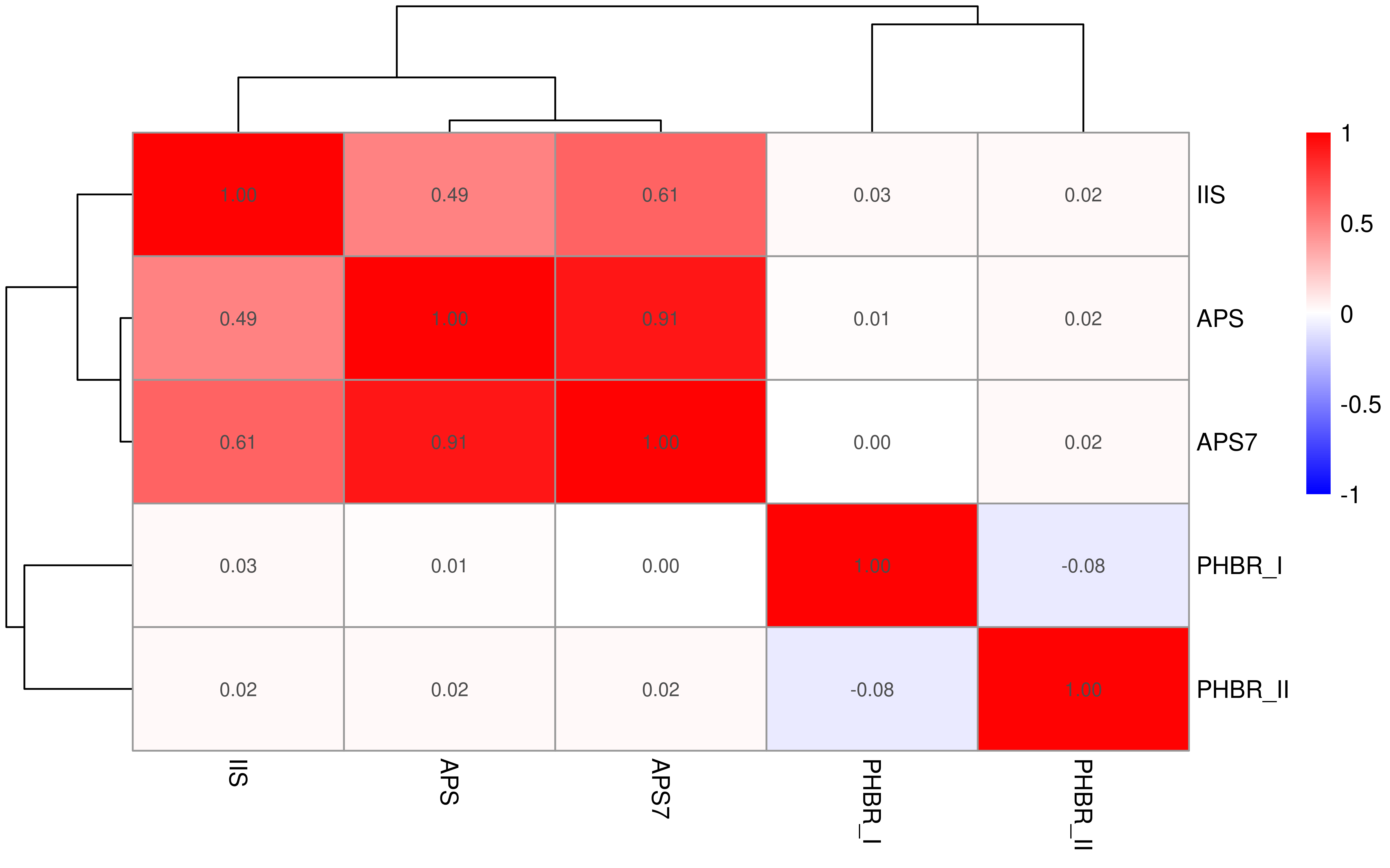
#> Joining, by = "Tumor_Sample_Barcode"Association between GSVA scores and other presentation scores
Here we explore association across APS, APS7, IIS, PHBR_I, PHBR_II.
First we check pan-cancer level association.
Show heatmap.
breaksList <- seq(-1, 1, by = 0.01)
colnames(cor_mat1)[colnames(cor_mat1) == "APM"] <- "APS"
rownames(cor_mat1)[rownames(cor_mat1) == "APM"] <- "APS"

pheatmap::pheatmap(cor_mat1,
  display_numbers = TRUE,
  color = colorRampPalette(c("blue", "white", "red"))(length(breaksList)),
  breaks = breaksList
)
Second we check cancer type specific level association.
cor_mat2 <- score_df %>%
  group_by(Project) %>%
  nest() %>%
  slice(1) %>%
  mutate(cor = map(data, cor, method = "spearman", use = "pairwise.complete.obs"))
Here we get 32 correlation matrixes.
cor_mat2
#> # A tibble: 32 x 3
#> # Groups:   Project [32]
#>    Project           data cor
#>    <chr>   <list<df[,5]>> <list>
#>  1 ACC           [92 × 5] <dbl[,5] [5 × 5]>
#>  2 BLCA         [412 × 5] <dbl[,5] [5 × 5]>
#>  3 BRCA       [1,087 × 5] <dbl[,5] [5 × 5]>
#>  4 CESC         [308 × 5] <dbl[,5] [5 × 5]>
#>  5 CHOL          [36 × 5] <dbl[,5] [5 × 5]>
#>  6 COAD         [462 × 5] <dbl[,5] [5 × 5]>
#>  7 DLBC          [48 × 5] <dbl[,5] [5 × 5]>
#>  8 ESCA         [185 × 5] <dbl[,5] [5 × 5]>
#>  9 GBM          [602 × 5] <dbl[,5] [5 × 5]>
#> 10 HNSC         [528 × 5] <dbl[,5] [5 × 5]>
#> # … with 22 more rows
Output the result pheatmaps to PDF is a good option to observe results.
# old.par <- par(mfrow=c(1, 2))
pdf("Score_correlation_matrix.pdf")

for (i in seq_len(nrow(cor_mat2))) {
  message("Processing ", cor_mat2$Project[i])
  colnames(cor_mat2$cor[[i]])[colnames(cor_mat2$cor[[i]]) == "APM"] <- "APS"
  rownames(cor_mat2$cor[[i]])[rownames(cor_mat2$cor[[i]]) == "APM"] <- "APS"
  print(pheatmap::pheatmap(cor_mat2$cor[[i]],
    display_numbers = TRUE,
    cluster_rows = FALSE, cluster_cols = FALSE,
    main = cor_mat2$Project[i],
    color = colorRampPalette(c("blue", "white", "red"))(length(breaksList)),
    breaks = breaksList
  ))
}
dev.off()
# par(old.par)
Association between subsets of immune cells and APS
Next we answer the question: which cells (CIBERSORT scores) or subsets of the IIS scores are most associated with the APS scores.
The first step is to calculate correlation using spearman method.
df.gsva.heat <- df.gsva.tumor %>%
  select(-c(Tumor_Sample_Barcode:Tumor_stage, APS7, IIS, TIS, PHBR_I, PHBR_II)) %>%
  filter(!is.na(APM)) %>%
  select(Project, APM, everything())
heat_mat <- sapply(unique(df.gsva.heat$Project), function(x) {
  mat <- filter(df.gsva.heat, Project == x)
  mat <- mat[, -1]
  cor_mat <- cor(mat, method = "spearman", use = "pairwise.complete.obs")
  cor_mat[, 1]
})
heat_mat <- heat_mat[-1, ]
Show plot.
library(pheatmap)
breaksList <- seq(-1, 1, by = 0.01)

pheatmap(heat_mat,
  color = colorRampPalette(c("blue", "white", "red"))(length(breaksList)),
  breaks = breaksList
)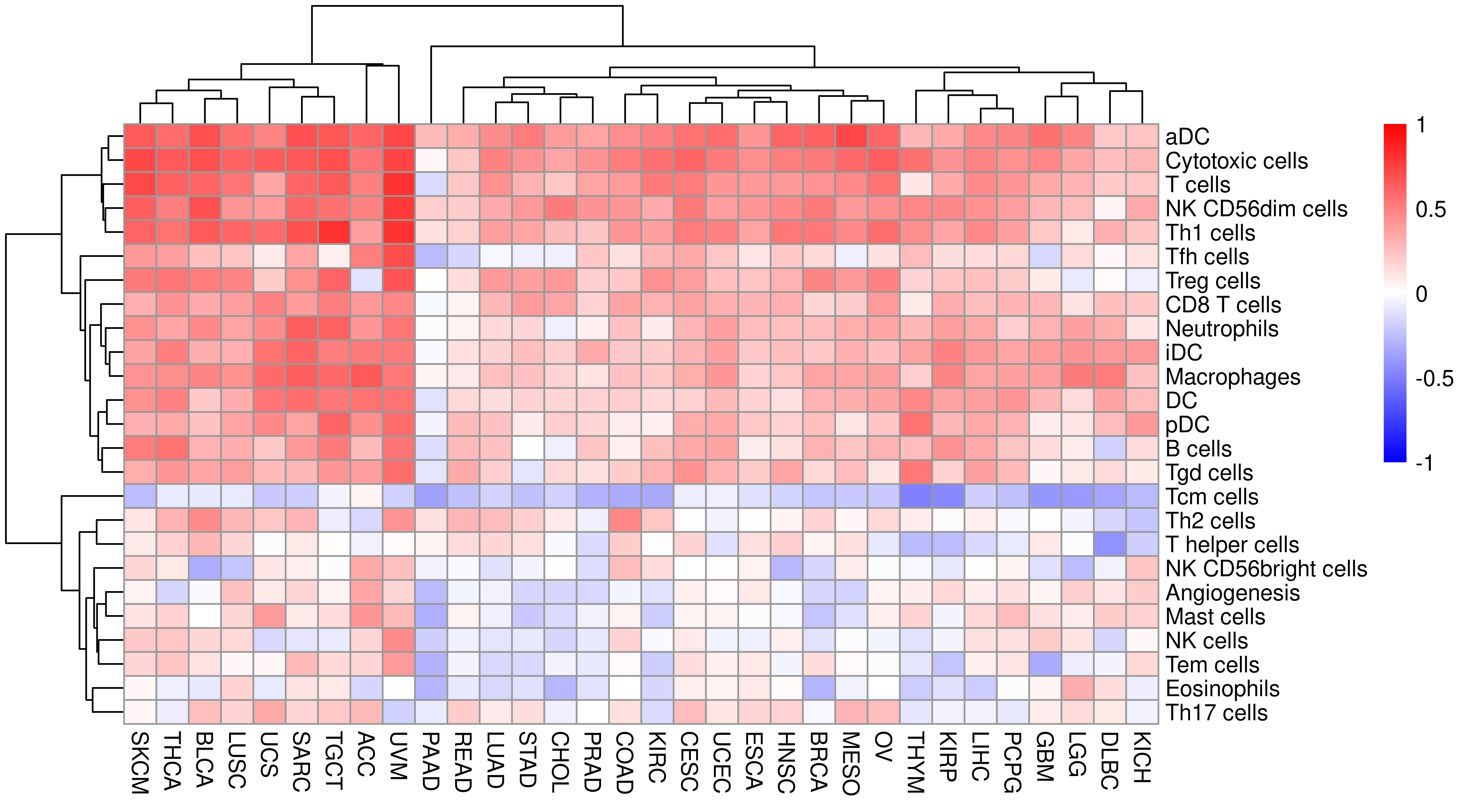
This shows that there is strong positive/consistent relationship between APM and immune/T cell infiltration level across TCGA cancer types. These spearman correlation coefficient are showed as a table.
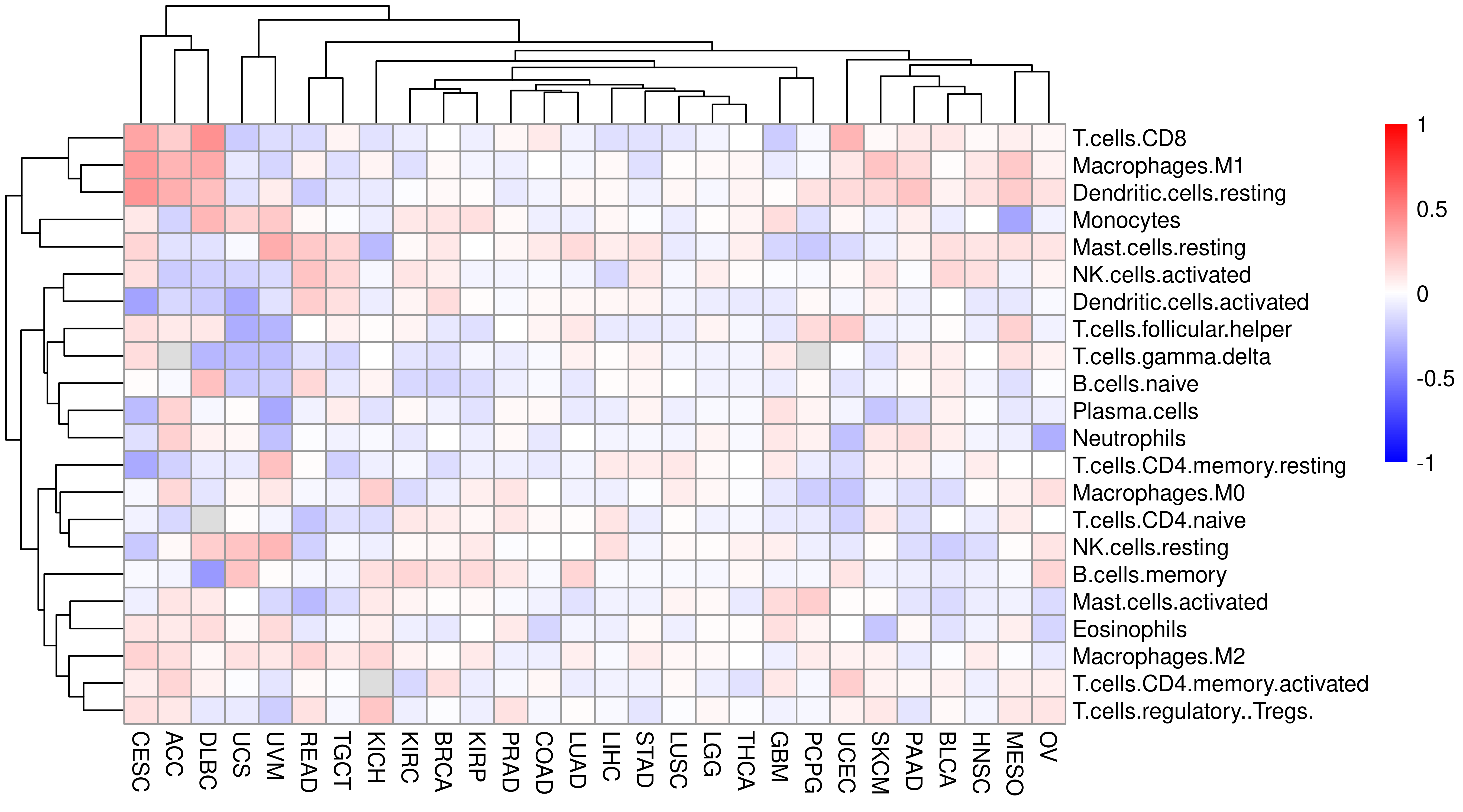
Thanks to TCGA, we can obtain CIBERSORT results for TCGA patients from paper The Immune Landscape of Cancer.
Combine APM (score) and CIBERSORT information, calculate correlation and plot heatmap.
cibersort_df <- left_join(
  df.gsva.tumor %>%
    select(Tumor_Sample_Barcode, Project, APM) %>%
    filter(!is.na(APM)),
  cibersort %>%
    select(-CancerType) %>%
    rename(Tumor_Sample_Barcode = SampleID) %>%
    mutate(Tumor_Sample_Barcode = substr(Tumor_Sample_Barcode, 1, 15)) %>%
    mutate(Tumor_Sample_Barcode = gsub("\\.", "-", Tumor_Sample_Barcode))
) %>% select(-c(Tumor_Sample_Barcode, P.value, Correlation, RMSE))
#> Joining, by = "Tumor_Sample_Barcode"
heat_mat2 <- sapply(unique(cibersort_df$Project), function(x) {
mat <- filter(cibersort_df, Project == x)
mat <- mat[, -1]
cor_mat <- cor(mat, method = "spearman", use = "pairwise.complete.obs")
cor_mat[, 1]
})
heat_mat2 <- heat_mat2[-1, ]pheatmap(heat_mat2,
color = colorRampPalette(c("blue", "white", "red"))(length(breaksList)),
breaks = breaksList
)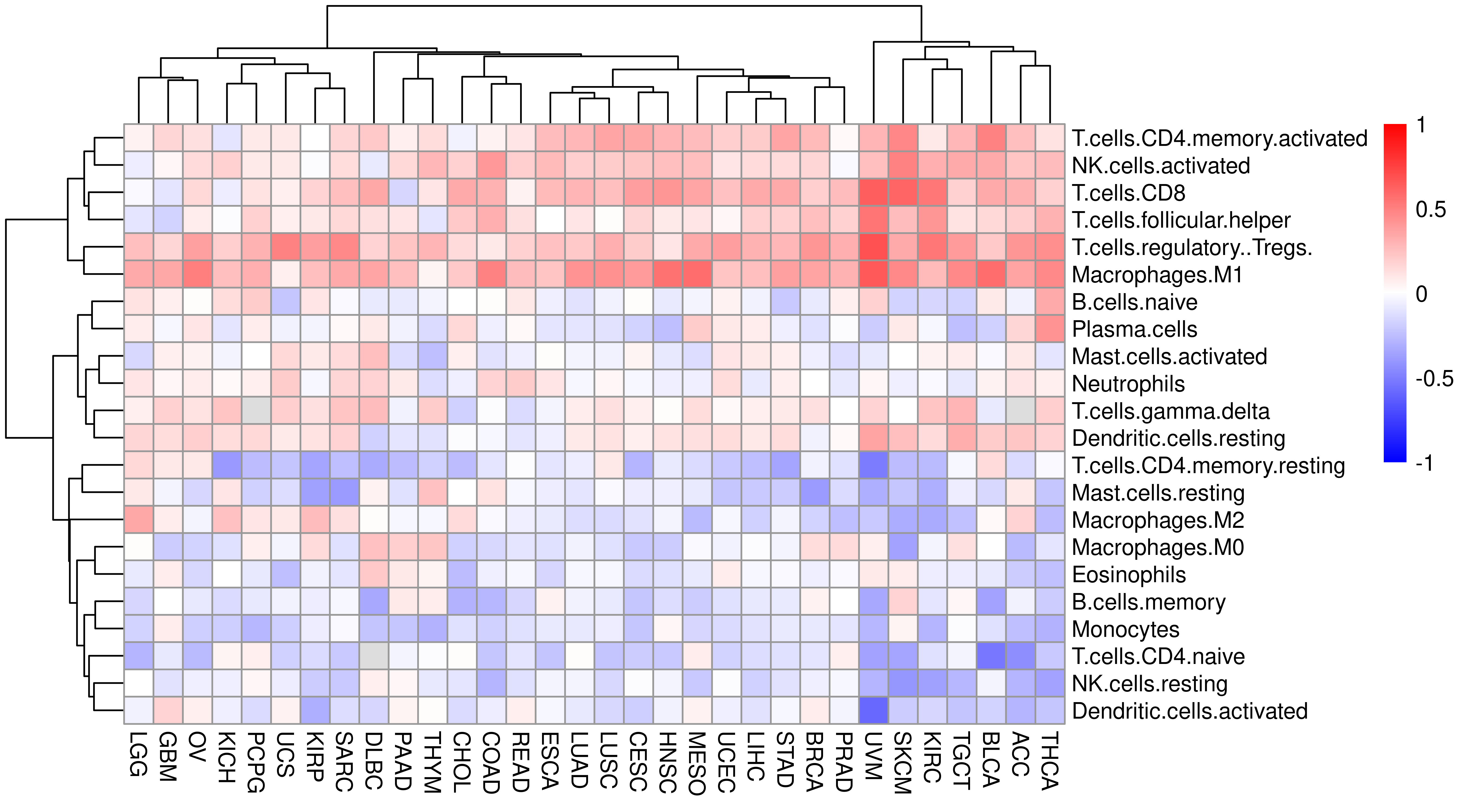
Indeed, APM score correlate with T cell infiltration.
However, we see PHBR_I, PHBR_II does not have relationship with either APS or IIS, does this score correlate with immune cell infiltration?
Let’s check it.
cibersort_df <- left_join(
  df.gsva.tumor %>%
    select(Tumor_Sample_Barcode, Project, PHBR_I) %>%
    filter(!is.na(PHBR_I)),
  cibersort %>%
    select(-CancerType) %>%
    rename(Tumor_Sample_Barcode = SampleID) %>%
    mutate(Tumor_Sample_Barcode = substr(Tumor_Sample_Barcode, 1, 15)) %>%
    mutate(Tumor_Sample_Barcode = gsub("\\.", "-", Tumor_Sample_Barcode))
) %>% select(-c(Tumor_Sample_Barcode, P.value, Correlation, RMSE))
#> Joining, by = "Tumor_Sample_Barcode"
heat_mat2 <- sapply(unique(cibersort_df$Project), function(x) {
mat <- filter(cibersort_df, Project == x)
mat <- mat[, -1]
cor_mat <- cor(mat, method = "spearman", use = "pairwise.complete.obs")
cor_mat[, 1]
})
heat_mat2 <- heat_mat2[-1, ]pheatmap(heat_mat2,
color = colorRampPalette(c("blue", "white", "red"))(length(breaksList)),
breaks = breaksList
)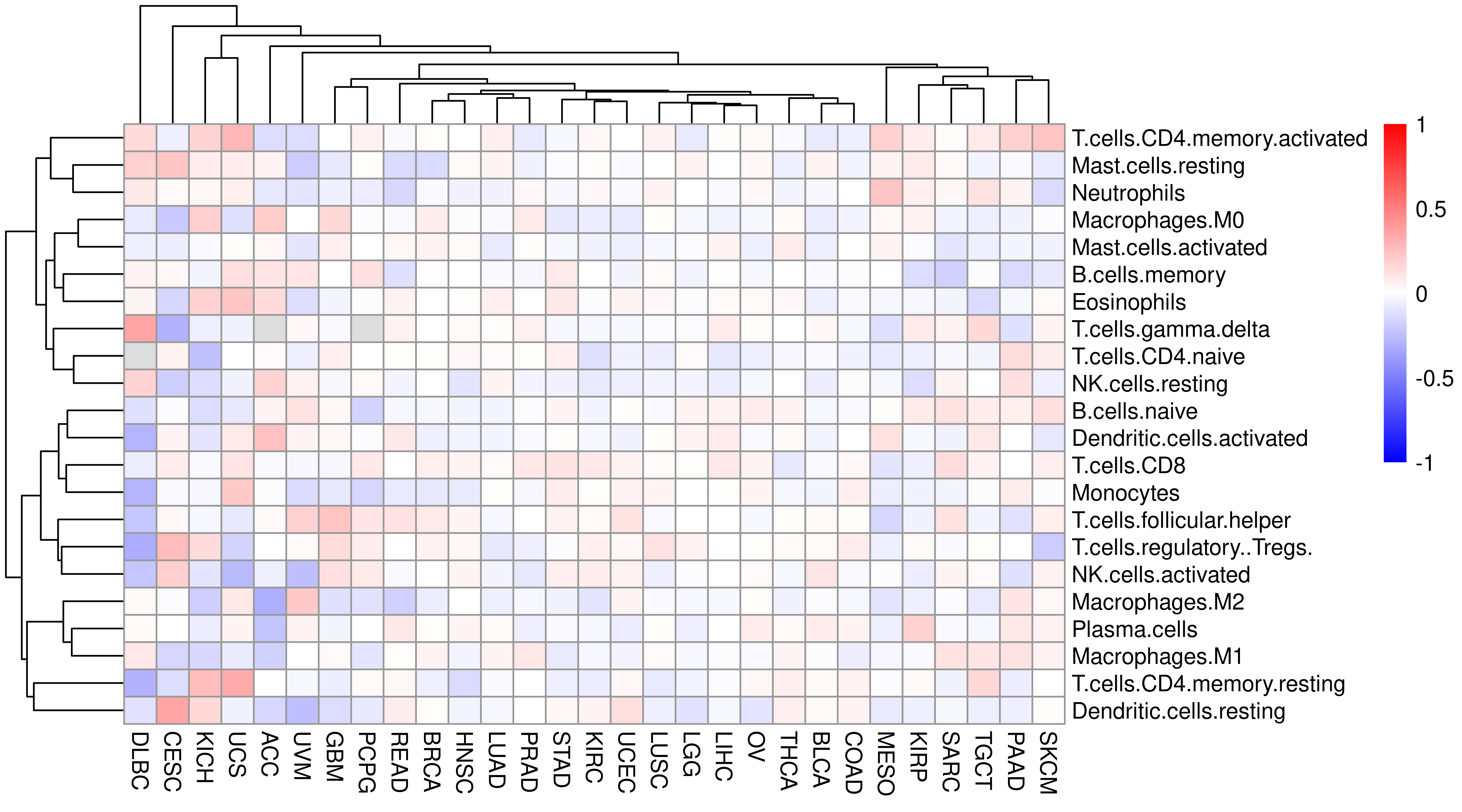
Do the same analysis for PHBR_II score.
cibersort_df <- left_join(
  df.gsva.tumor %>%
    select(Tumor_Sample_Barcode, Project, PHBR_II) %>%
    filter(!is.na(PHBR_II)),
  cibersort %>%
    select(-CancerType) %>%
    rename(Tumor_Sample_Barcode = SampleID) %>%
    mutate(Tumor_Sample_Barcode = substr(Tumor_Sample_Barcode, 1, 15)) %>%
    mutate(Tumor_Sample_Barcode = gsub("\\.", "-", Tumor_Sample_Barcode))
) %>% select(-c(Tumor_Sample_Barcode, P.value, Correlation, RMSE))
#> Joining, by = "Tumor_Sample_Barcode"
heat_mat2 <- sapply(unique(cibersort_df$Project), function(x) {
mat <- filter(cibersort_df, Project == x)
mat <- mat[, -1]
cor_mat <- cor(mat, method = "spearman", use = "pairwise.complete.obs")
cor_mat[, 1]
})
heat_mat2 <- heat_mat2[-1, ]pheatmap(heat_mat2,
color = colorRampPalette(c("blue", "white", "red"))(length(breaksList)),
breaks = breaksList
)
IIS is a good representation of immune cell infiltration
Immune/T cell infiltration is a good indicator for ICB response. Here we have seen that APS have strong association with both TIS and IIS. In indivial level, i.e. 9095 samples, we also observe that TIS and IIS are basically same because their correlation coeficient is about 0.91!
df.gsva.tumor %>%
  filter(!is.na(IIS)) %>%
  summarise(corr = cor(TIS, IIS, method = "spearman"))
#> # A tibble: 1 x 1
#>    corr
#>   <dbl>
#> 1 0.909
Therefore, we should choose one of them for downstream analysis. Finally, we choose IIS not only because it is more comprehensive, but also it is well validated.
- In vitro validation with multiplex immunofluorescence, in silico validation using simulated mixing proportions and comparison between CIBERSORT and IIS have been previously described (Senbabaoglu, Y. et al).
TIMER is another method that can accurately resolve relative fractions of diverse cell types based on gene expression profiles from complex tissues. To further validate the calculated IIS, we perform TIMER analysis and find that the result of TIMER is highly correlated with the calculated IIS.
load("results/timer.RData")

df <- dplyr::select(df.gsva.tumor, Project, APM, IIS, APS7, PHBR_I, PHBR_II, Gender, Age, Tumor_stage, OS.time, OS, Tumor_Sample_Barcode)

df_timer <- dplyr::left_join(x = df, y = timer_clean, by = c("Tumor_Sample_Barcode" = "sample"))library(corrplot)
mat_timer_IIS <- df_timer %>%
select(-c(APM, APS7, PHBR_I, PHBR_II, Gender:Tumor_Sample_Barcode)) %>%
filter(!is.na(IIS) & !is.na(T_cell.CD8)) %>%
filter(T_cell.CD8 != 0)
mat_timer_IIS.heat <- sapply(unique(mat_timer_IIS$Project), function(x) {
mat <- filter(mat_timer_IIS, Project == x)
mat <- mat[, -1]
cor_mat <- cor(mat, method = "spearman", use = "pairwise.complete.obs")
cor_mat[, 1]
})
mat_timer_IIS.heat <- mat_timer_IIS.heat[-1, -22]
p.mat <- sapply(unique(mat_timer_IIS$Project), function(x) {
mat <- filter(mat_timer_IIS, Project == x)
mat <- mat[, -1]
tryCatch(expr = {
p_mat <- cor.mtest(mat, method = "spearman", conf.level = .95)
p_mat[[1]][, 1]
}, error = function(e) {
rep(NA, 7)
})
})
p.mat <- p.mat[-1, -22]
col <- colorRampPalette(c("blue", "white", "red"))(200)
corrplot(mat_timer_IIS.heat,
method = "color", tl.col = "black", tl.srt = 45,
col = col, p.mat = p.mat, sig.level = 0.05
)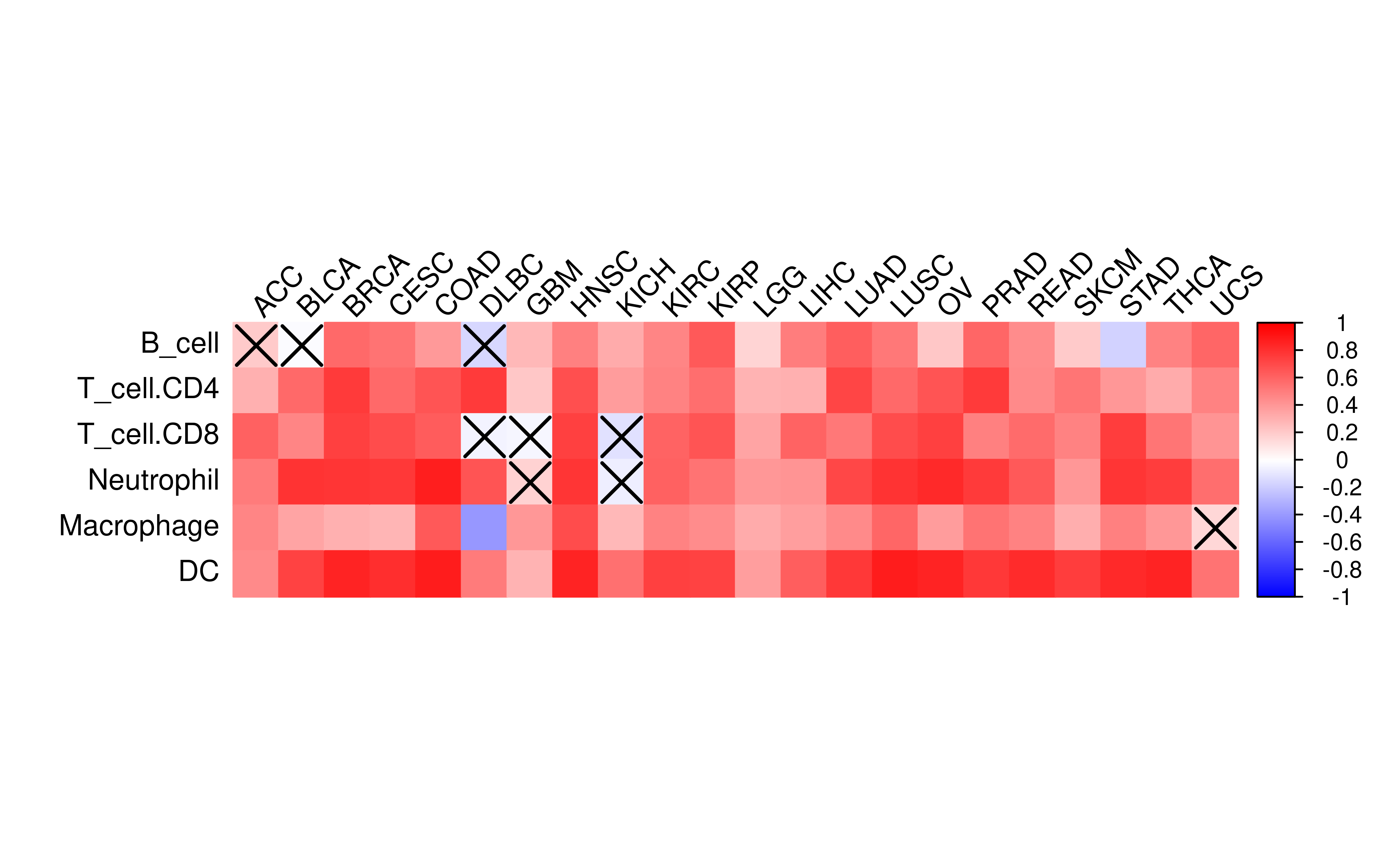
The color bar in figure shows correlation coefficient values. The “X” marks relationship does not pass significant test (i.e. p>=0.05).
Even Senbabaoglu et al have checked the relationship between IIS and CIBERSORT in clear cell renal cell carcinoma. Here we expand it to all TCGA cancer type with CIBERSORT data and IIS avaiable.
df_cibersort <- left_join(
  df.gsva.tumor %>%
    select(Tumor_Sample_Barcode, Project, IIS) %>%
    filter(!is.na(IIS)),
  cibersort %>%
    select(-CancerType) %>%
    rename(Tumor_Sample_Barcode = SampleID) %>%
    mutate(Tumor_Sample_Barcode = substr(Tumor_Sample_Barcode, 1, 15)) %>%
    mutate(Tumor_Sample_Barcode = gsub("\\.", "-", Tumor_Sample_Barcode))
) %>% select(-c(Tumor_Sample_Barcode, P.value, Correlation, RMSE))
#> Joining, by = "Tumor_Sample_Barcode"
mat_cibersort_IIS.heat <- sapply(unique(df_cibersort$Project), function(x) {
  mat <- filter(df_cibersort, Project == x)
  mat <- mat[, -1]
  cor_mat <- cor(mat, method = "spearman", use = "pairwise.complete.obs")
  cor_mat[, 1]
})

pheatmap(heat_mat2[-1, ],
  color = colorRampPalette(c("blue", "white", "red"))(length(breaksList)),
  breaks = breaksList
)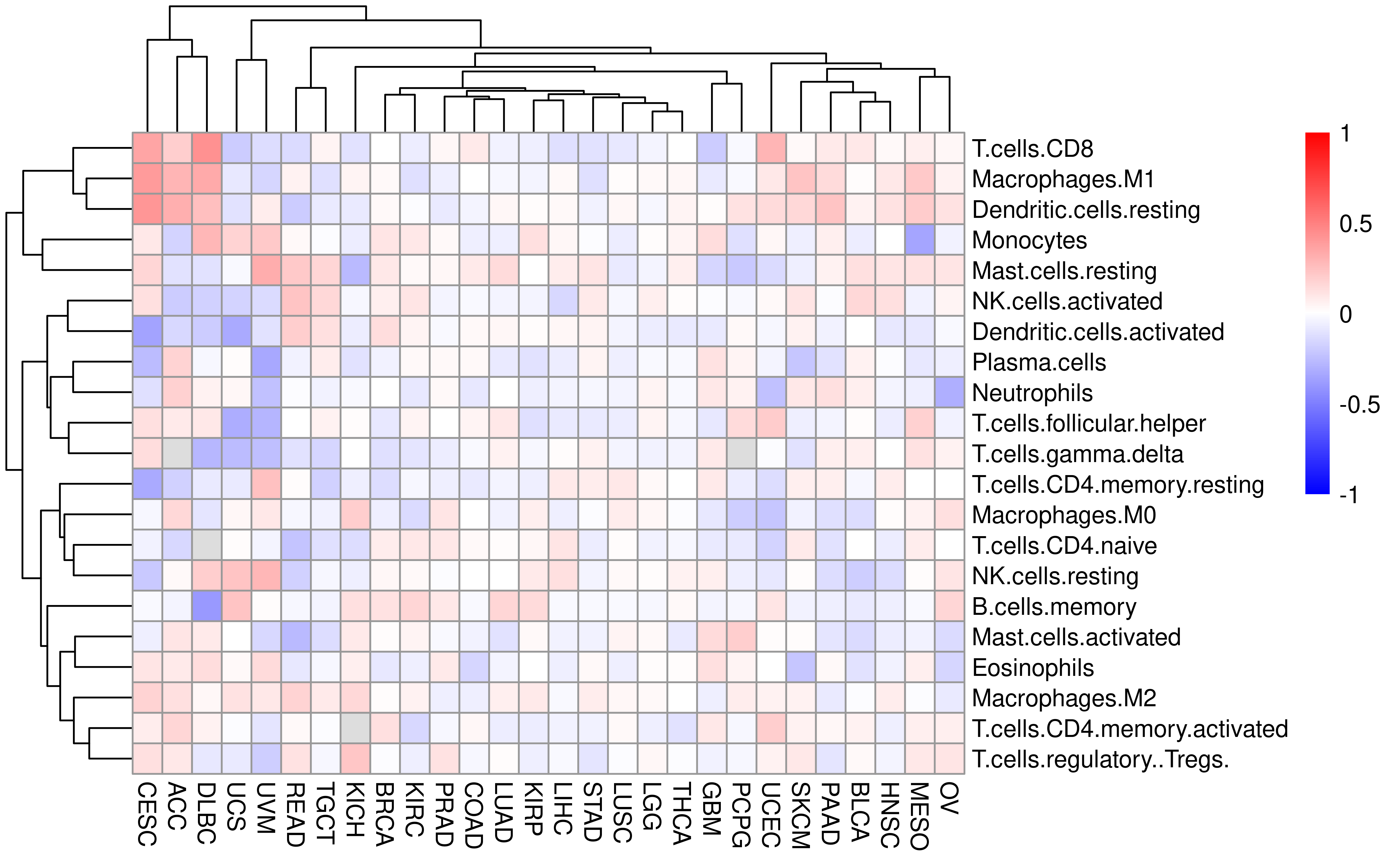
Compare with timer, the relationship between IIS and immune cell subsets is more variable. I think this can be explained by several reasons:
- CIBERSORT and TIMER target different aspects of tumor immune infiltrates. CIBERSORT infers the relative fractions of immune subsets in the total leukocyte population, while TIMER predicts the abundance of immune cells in the overall tumor microenvironment. Currently both methods are limited by the assumption that transcriptomes of tumor-infiltrating immune cells do not significantly differ from those collected from peripheral blood of healthy donors. (This is from Revisit linear regression-based deconvolution methods for tumor gene expression data)
- Many cibersort values are equal to 0 or close to 0, this reduce the power to calculate correlation
- CIBERSORT predicts 22 immune cell subsets while TIMER obtains 6 cell types, it is not unexpected to observe a more variable result using CIBERSORT.
Exploration of APS, TMB, TIGS at pan-cancer level
Load TCGA TMB data and merge all necessary datasets.
load("results/TCGA_TMB.RData")

df2 <- df %>%
  mutate(Tumor_Sample_Barcode = substr(Tumor_Sample_Barcode, 1, 12)) %>%
  arrange(APM) %>%
  distinct(Tumor_Sample_Barcode, .keep_all = TRUE)
tcga_all <- full_join(df2, TCGA_TMB, by = "Tumor_Sample_Barcode")

if (!file.exists("results/TCGA_ALL.RData")) {
  save(tcga_all, file = "results/TCGA_ALL.RData")
}

rm(list = ls())
Tumor mutation burden (TMB) is defined as the number of non-synonymous alterations per megabase (Mb) of genome examined. As reported previously, here we use 38 Mb as the estimate of the exome size. For studies reporting mutation number from whole exome sequencing, the normalized TMB = (whole exome non-synonymous mutation)/(38 Mb).
Original APM scores (APS) from GSVA are in the range of -1 to 1. To calculate tumor immunogenicity score (TIGS), original APM score from GSVA implementation is rescaled by minimal and maximal APM score from TCGA Pan-cancer analysis.
We calculate tumor immunogenicity score (TIGS) as following:
\[ TIGS = APS_{normalized} \times log(TMB + 1) \]
Natural logarithm is applied here. Of note, some tumors have TMB level below 1 mutation/ Mb, to avoid minus number in quantifying “tumor antigenicity”, we add number 1 to all normalized TMB.
How we generate this TIGS formula will be described at an individual part. Here we focus on association of APS, TMB and TIGS and their effects.
load("results/TCGA_ALL.RData")

tcga_all <- tcga_all %>%
  mutate(
    nAPM = (APM - min(APM, na.rm = TRUE)) / (max(APM, na.rm = TRUE) - min(APM, na.rm = TRUE)),
    nTMB = TMB_NonsynVariants / 38,
    TIGS = log(nTMB + 1) * nAPM
  ) %>%
  rename(Event = OS, Time = OS.time)


# keep samples with survival information
df_os <- tcga_all %>%
  filter(!is.na(Time), !is.na(Event))


df_os %>%
  filter(!is.na(nAPM)) %>%
  group_by(Project) %>%
  summarise(N = n()) %>%
  arrange(N)
#> # A tibble: 32 x 2
#>    Project     N
#>    <chr>   <int>
#>  1 CHOL       36
#>  2 DLBC       47
#>  3 UCS        56
#>  4 KICH       65
#>  5 ACC        79
#>  6 UVM        80
#>  7 MESO       85
#>  8 READ       92
#>  9 SKCM      102
#> 10 THYM      119
#> # … with 22 more rows

df_os %>%
  filter(!is.na(TIGS)) %>%
  group_by(Project) %>%
  summarise(N = n()) %>%
  arrange(N)
#> # A tibble: 32 x 2
#>    Project     N
#>    <chr>   <int>
#>  1 CHOL       36
#>  2 DLBC       36
#>  3 UCS        56
#>  4 KICH       65
#>  5 ACC        79
#>  6 MESO       80
#>  7 UVM        80
#>  8 READ       89
#>  9 SKCM      102
#> 10 THYM      118
#> # … with 22 more rows
Distribution of APS, TMB and IIS across TCGA studies
Calculate median values to sort distribution.
#------------ TIGS, TMB, APM pancan, sort by value
df_summary <- df_os %>%
  group_by(Project) %>%
  summarise(
    medianAPM = median(APM, na.rm = TRUE),
    medianTMB = median(TMB_NonsynVariants, na.rm = TRUE),
    medianTIGS = median(TIGS, na.rm = TRUE),
    medianAPMn = median(nAPM, na.rm = TRUE),
    medianTMBn = log(median(nTMB, na.rm = TRUE) + 1)
  )
Distribution of APM score (APS) across TCGA studies.
library(scales)
library(ggpubr)

df_os %>%
  filter(!is.na(Project), !is.na(APM)) %>%
  ggboxplot(
    x = "Project", y = "APM", color = "Project", add = "jitter", xlab = "TCGA Projects",
    ylab = "APM Score", add.params = list(size = 0.6),
    legend = "none"
  ) +
  rotate_x_text(angle = 45) +
  geom_hline(yintercept = mean(df_os$APM, na.rm = TRUE), linetype = 2) +
  scale_x_discrete(limits = arrange(df_summary, medianAPM) %>% .$Project) -> p_apm
p_apm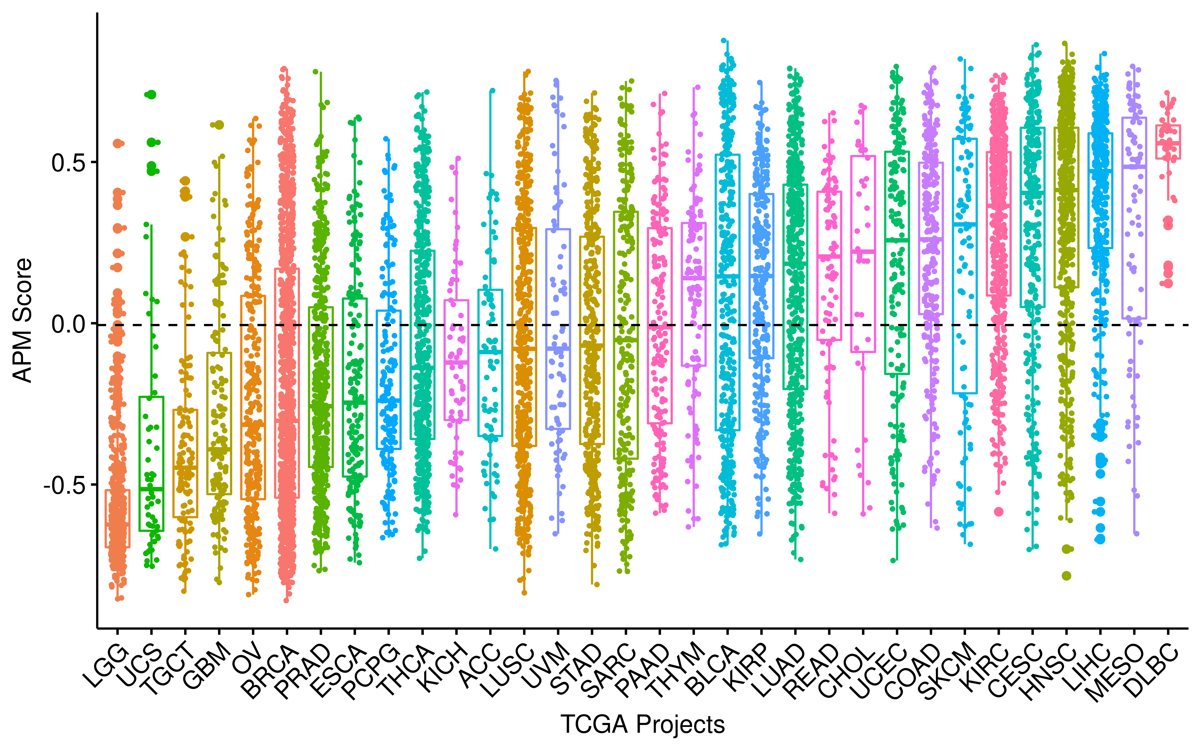
Distribution of TMB across TCGA studies.
df_os %>%
  filter(!is.na(Project), !is.na(TMB_NonsynVariants)) %>%
  ggboxplot(
    x = "Project", y = "TMB_NonsynVariants", color = "Project", add = "jitter", xlab = "TCGA Projects",
    ylab = "No. of Coding Somatic Nonsynonymous Mutation", add.params = list(size = 0.6),
    legend = "none"
  ) +
  rotate_x_text(angle = 45) +
  geom_hline(yintercept = mean(df_os$TMB_NonsynVariants, na.rm = TRUE), linetype = 2) +
  scale_y_log10(breaks = 10^(-1:4), labels = trans_format("log10", math_format(10^.x))) +
  scale_x_discrete(limits = arrange(df_summary, medianTMB) %>% .$Project) -> p_tmb
p_tmb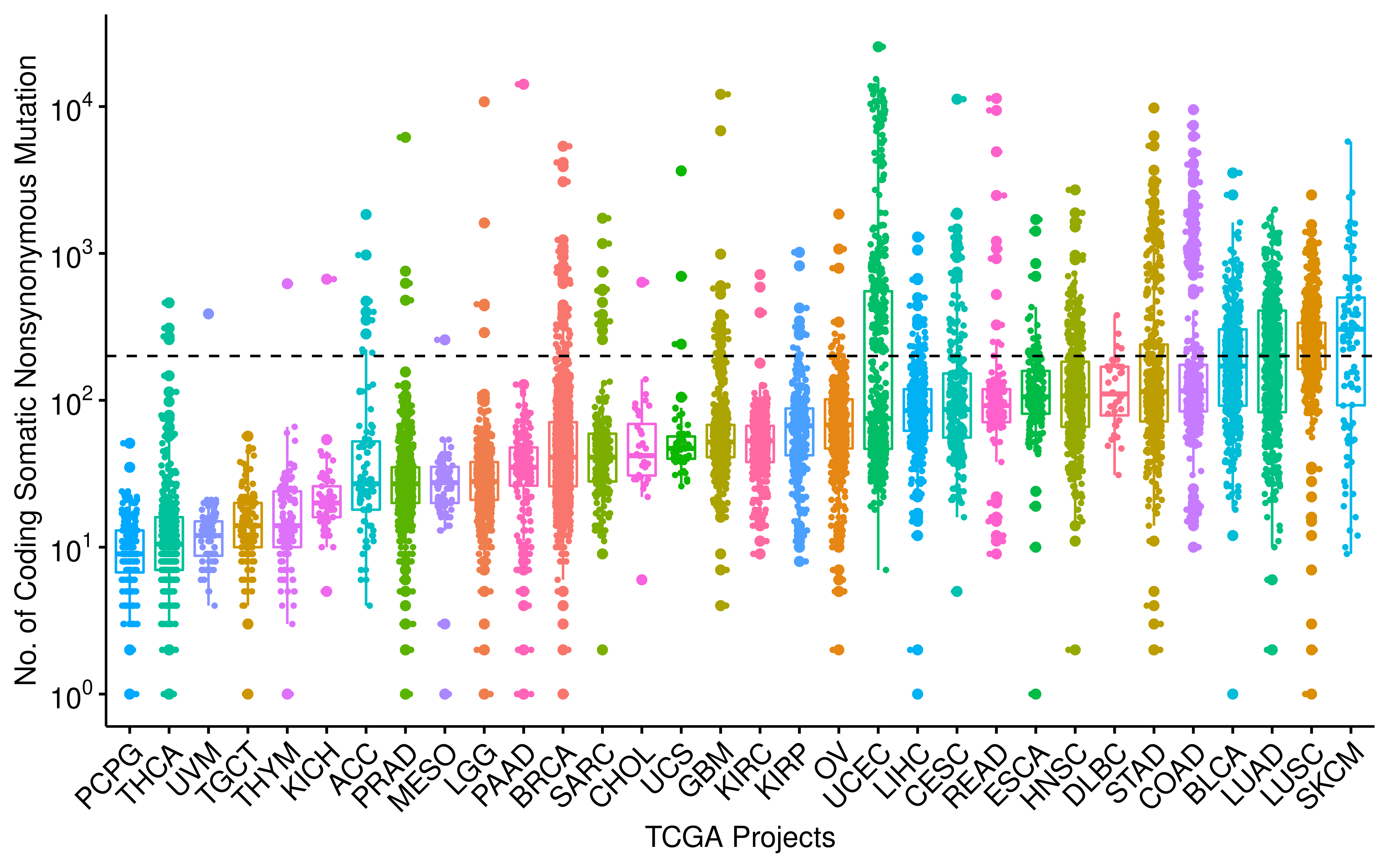
Distribution of TIGS across TCGA studies.
df_os %>%
  filter(!is.na(Project), !is.na(TIGS)) %>%
  ggboxplot(
    x = "Project", y = "TIGS", color = "Project", add = "jitter", xlab = "TCGA Projects",
    ylab = "TIGS", add.params = list(size = 0.6),
    legend = "none"
  ) +
  rotate_x_text(angle = 45) +
  geom_hline(yintercept = mean(df_os$TIGS, na.rm = TRUE), linetype = 2) +
  scale_x_discrete(limits = arrange(df_summary, medianTIGS) %>% .$Project) -> p_tigs
p_tigs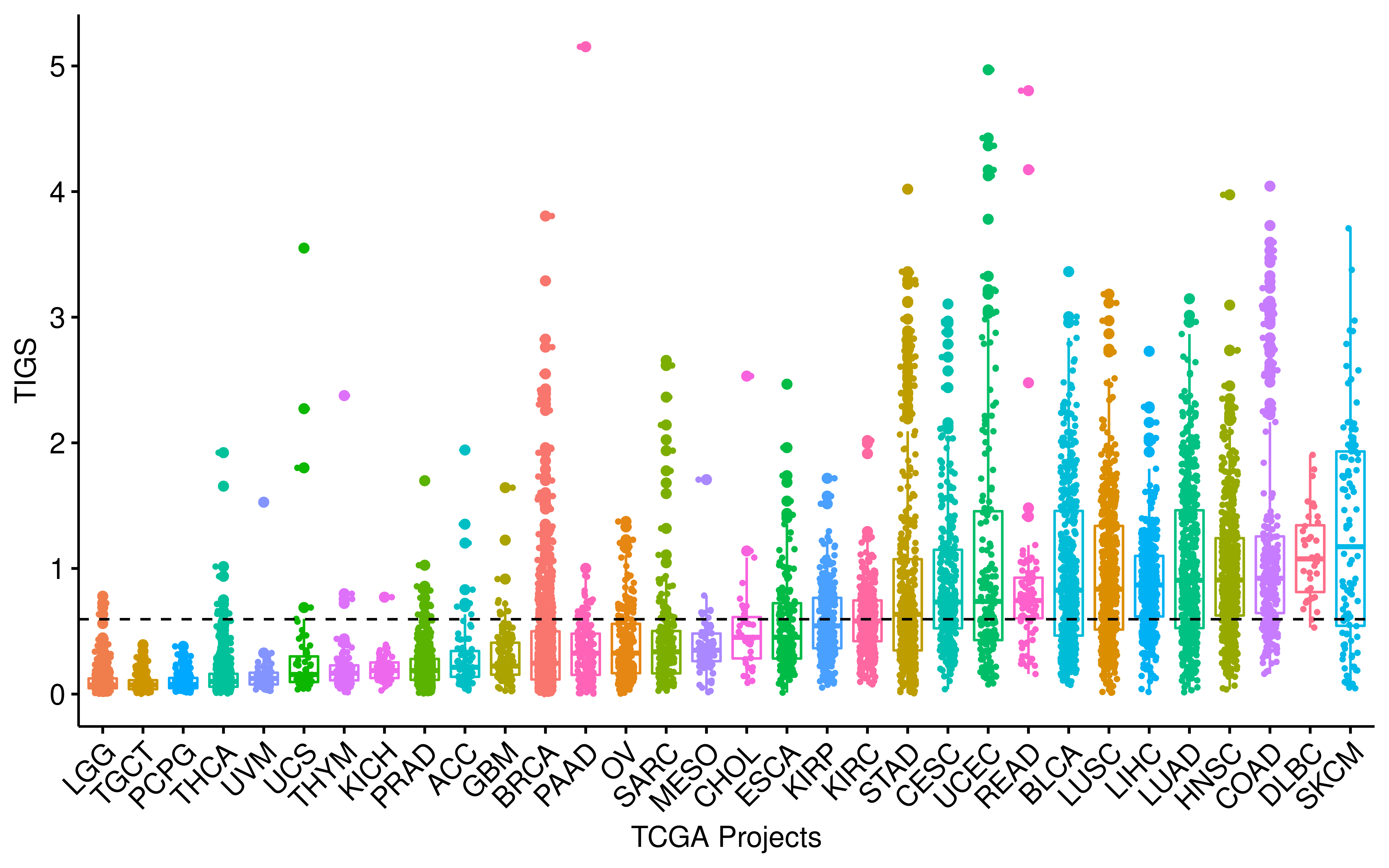
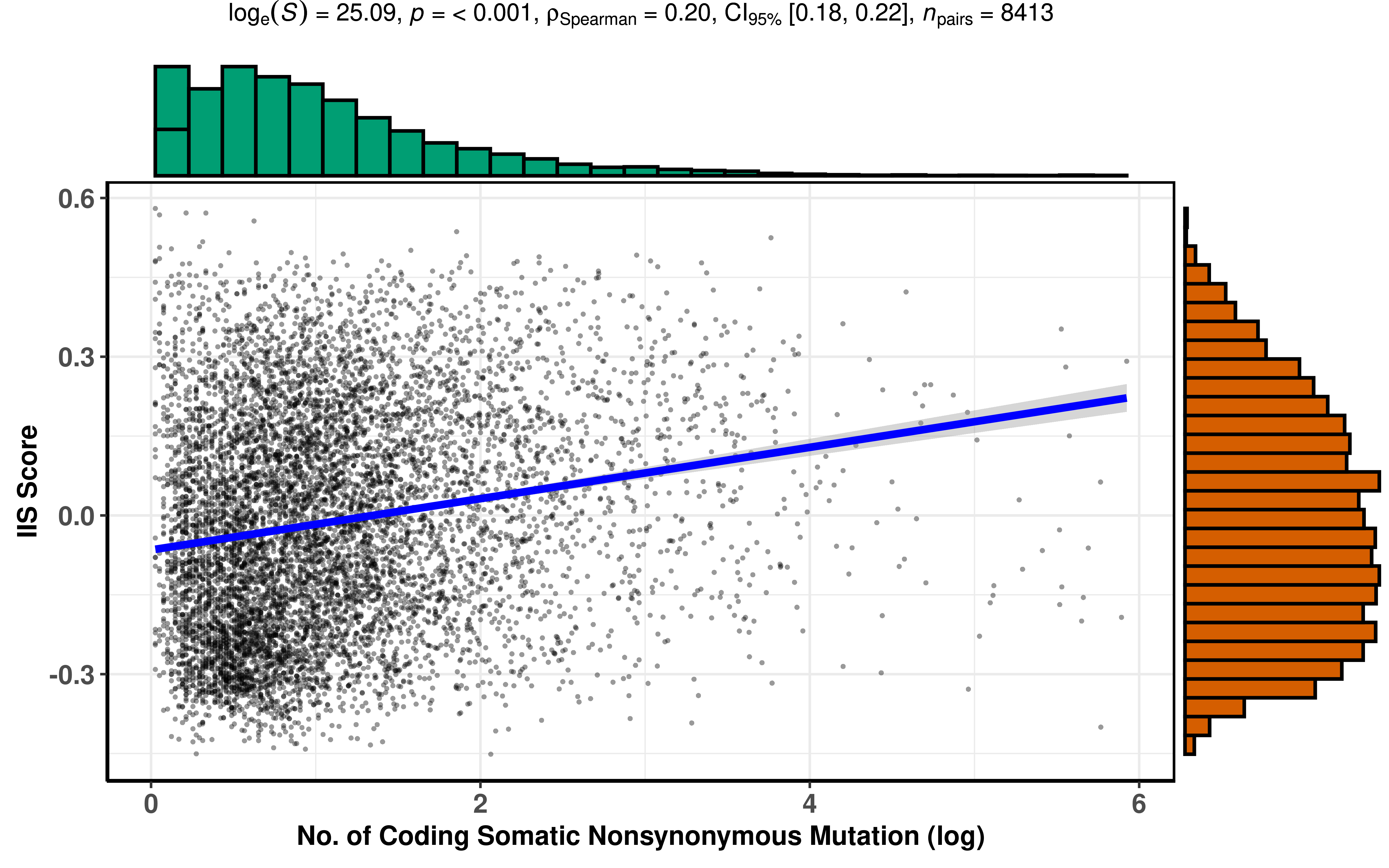
Correlation between TMB and IIS
df_TMB <- df_os %>%
  filter(!is.na(IIS), !is.na(TMB_NonsynVariants)) %>%
  mutate(logTMB = log(nTMB + 1))

ggstatsplot::ggscatterstats(
  data = df_TMB,
  x = nTMB,
  y = IIS,
  xlab = "No. of Coding Somatic Nonsynonymous Mutation",
  ylab = "IIS Score",
  point.size = 1,
  # title = "Correlation between APM and IIS score in pancancer",
  messages = FALSE, type = "spearman"
)
#> Registered S3 methods overwritten by 'broom.mixed':
#>   method         from
#>   augment.lme    broom
#>   augment.merMod broom
#>   glance.lme     broom
#>   glance.merMod  broom
#>   glance.stanreg broom
#>   tidy.brmsfit   broom
#>   tidy.gamlss    broom
#>   tidy.lme       broom
#>   tidy.merMod    broom
#>   tidy.rjags     broom
#>   tidy.stanfit   broom
#>   tidy.stanreg   broom
#> Registered S3 methods overwritten by 'survival':
#>   method       from
#>   nobs.coxph   insight
#>   nobs.survreg insight
#> Registered S3 methods overwritten by 'car':
#>   method                          from
#>   influence.merMod                lme4
#>   cooks.distance.influence.merMod lme4
#>   dfbeta.influence.merMod         lme4
#>   dfbetas.influence.merMod        lme4


ggstatsplot::ggscatterstats(
  data = df_TMB,
  x = logTMB,
  y = IIS,
  xlab = "No. of Coding Somatic Nonsynonymous Mutation (log)",
  ylab = "IIS Score",
  point.size = 1,
  # title = "Correlation between APM and IIS score in pancancer",
  messages = FALSE, type = "spearman"
)
plot_scatter <- function(data, x, y, xlab = "Median APM", ylab = "Median IIS", conf.int = TRUE, method = "spearman", label.x = -0.5, label.y = 0.2, label = "Project", ...) {
  ggscatter(data,
    x = x, y = y,
    xlab = xlab, ylab = ylab,
    shape = 21, size = 3, color = "black",
    add = "reg.line", add.params = list(color = "blue", fill = "lightgray"),
    conf.int = conf.int,
    cor.coef = TRUE,
    cor.coeff.args = list(method = method, label.x = label.x, label.y = label.y, label.sep = "\n"),
    label = label, repel = TRUE, ...
  )
}

df_project <- df_TMB %>%
  group_by(Project) %>%
  summarise(
    TMB_median = median(nTMB, na.rm = TRUE),
    IIS_median = median(IIS, na.rm = TRUE)
  )

mean(df_TMB$nTMB)
#> [1] 4.307116
plot_scatter(df_project,
  x = "TMB_median", y = "IIS_median",
  xlab = "Median TMB", ylab = "Median IIS", label.x = 0.2
) +
  geom_hline(yintercept = 0, linetype = 2) + geom_vline(xintercept = 4.35, linetype = 2)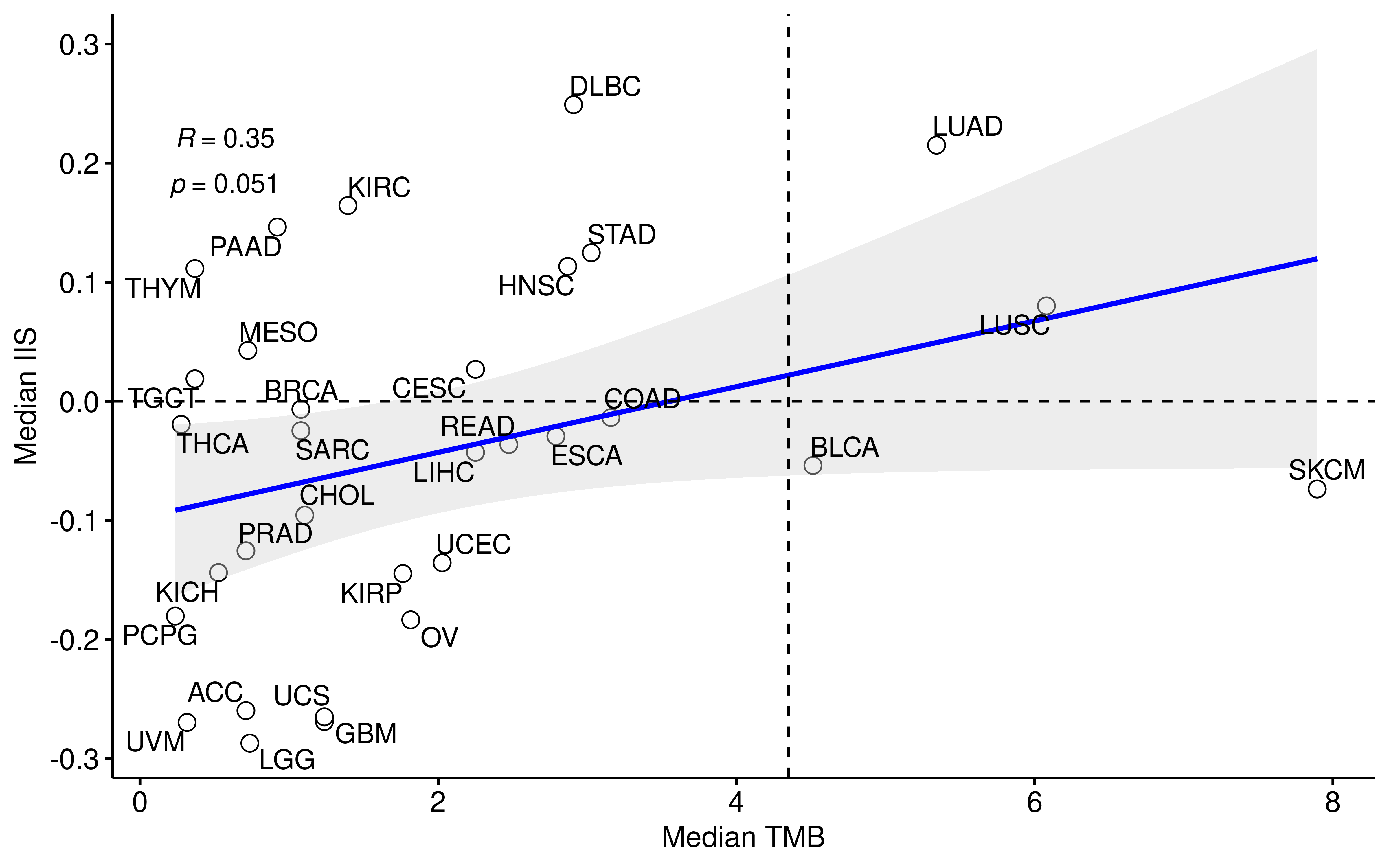
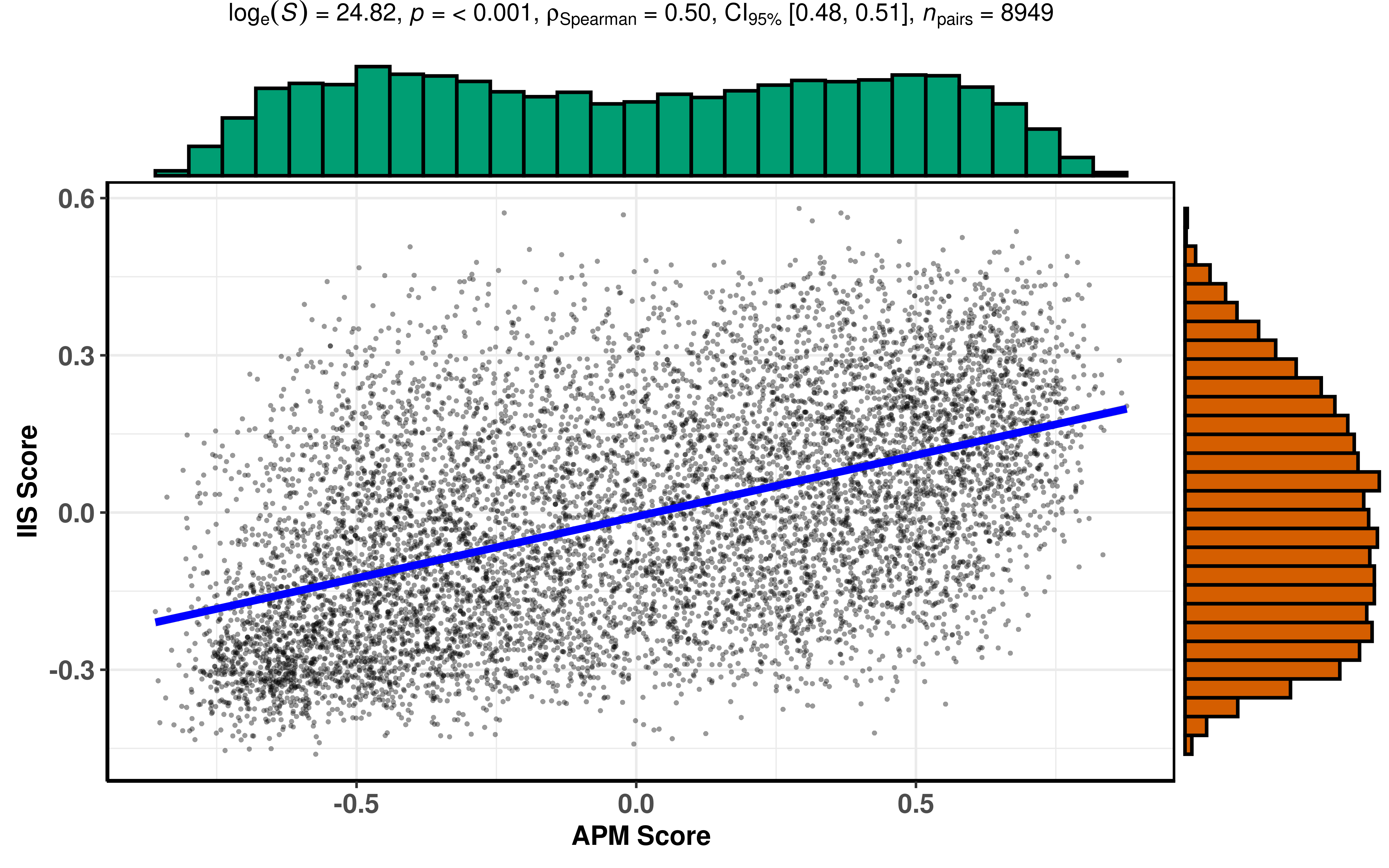
Significant correlation between APM score and IIS
ggstatsplot::ggscatterstats(
  data = df_os %>% filter(!is.na(APM)),
  x = APM,
  y = IIS,
  xlab = "APM Score",
  ylab = "IIS Score",
  point.size = 1,
  # title = "Correlation between APM and IIS score in pancancer",
  messages = FALSE, type = "spearman"
)
df_project2 <- df_os %>%
  filter(!is.na(APM)) %>%
  group_by(Project) %>%
  summarise(
    APM_median = median(APM),
    IIS_median = median(IIS)
  )

plot_scatter(df_project2,
  x = "APM_median", y = "IIS_median",
  xlab = "Median APM", ylab = "Median IIS"
) +
  geom_hline(yintercept = 0, linetype = 2) + geom_vline(xintercept = 0, linetype = 2)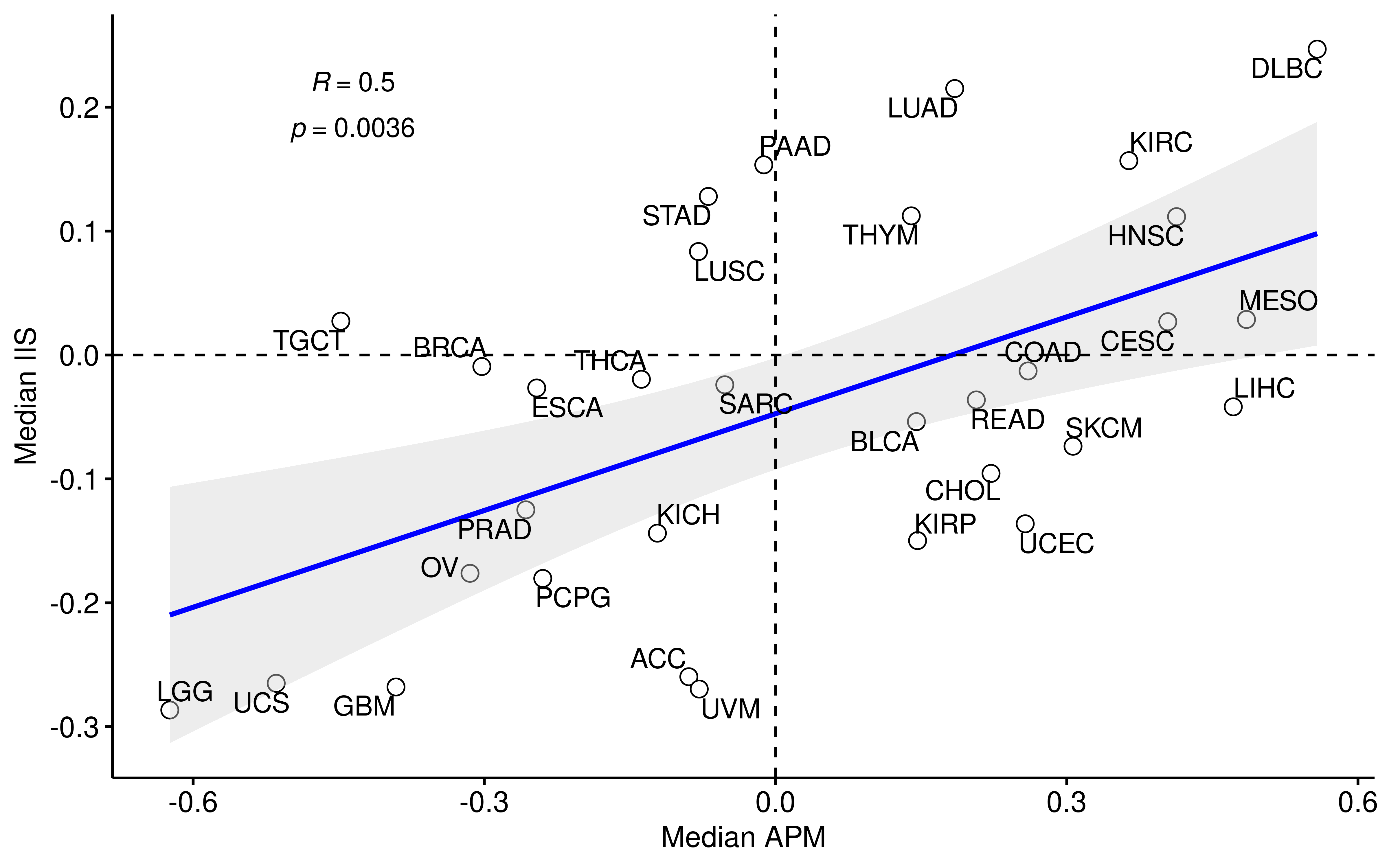
Survival analysis
Check pan-cancer level influence of APS, TMB and TIGS using unvariable cox model.
library(survival)
fit_APS <- coxph(Surv(Time, Event) ~ nAPM, data = filter(df_os, !is.na(nAPM)))
fit_TMB <- coxph(Surv(Time, Event) ~ log(nTMB), data = filter(df_os, !is.na(nTMB)))
fit_TIGS <- coxph(Surv(Time, Event) ~ TIGS, data = filter(df_os, !is.na(TIGS)))
fit_APS
#> Call:
#> coxph(formula = Surv(Time, Event) ~ nAPM, data = filter(df_os,
#> !is.na(nAPM)))
#>
#> coef exp(coef) se(coef) z p
#> nAPM 0.37300 1.45208 0.07837 4.759 1.94e-06
#>
#> Likelihood ratio test=22.69 on 1 df, p=1.9e-06
#> n= 8949, number of events= 2589
fit_TMB
#> Call:
#> coxph(formula = Surv(Time, Event) ~ log(nTMB), data = filter(df_os,
#> !is.na(nTMB)))
#>
#> coef exp(coef) se(coef) z p
#> log(nTMB) 0.17413 1.19021 0.01306 13.33 <2e-16
#>
#> Likelihood ratio test=167.4 on 1 df, p=< 2.2e-16
#> n= 9476, number of events= 2781
fit_TIGS
#> Call:
#> coxph(formula = Surv(Time, Event) ~ TIGS, data = filter(df_os,
#> !is.na(TIGS)))
#>
#> coef exp(coef) se(coef) z p
#> TIGS 0.29631 1.34488 0.02858 10.37 <2e-16
#>
#> Likelihood ratio test=94.47 on 1 df, p=< 2.2e-16
#> n= 8413, number of events= 2365dplyr::tibble(
Variable = c("APS", "TMB", "TIGS"),
N = c(summary(fit_APS)$n, summary(fit_TMB)$n, summary(fit_TIGS)$n),
Coef = c(summary(fit_APS)$conf.int[1], summary(fit_TMB)$conf.int[1], summary(fit_TIGS)$conf.int[1]),
Lower = c(summary(fit_APS)$conf.int[3], summary(fit_TMB)$conf.int[3], summary(fit_TIGS)$conf.int[3]),
Upper = c(summary(fit_APS)$conf.int[4], summary(fit_TMB)$conf.int[4], summary(fit_TIGS)$conf.int[4]),
P.value = c(summary(fit_APS)$logtest[3], summary(fit_TMB)$logtest[3], summary(fit_TIGS)$logtest[3])
)
#> # A tibble: 3 x 6
#> Variable N Coef Lower Upper P.value
#> <chr> <int> <dbl> <dbl> <dbl> <dbl>
#> 1 APS 8949 1.45 1.25 1.69 1.90e- 6
#> 2 TMB 9476 1.19 1.16 1.22 2.78e-38
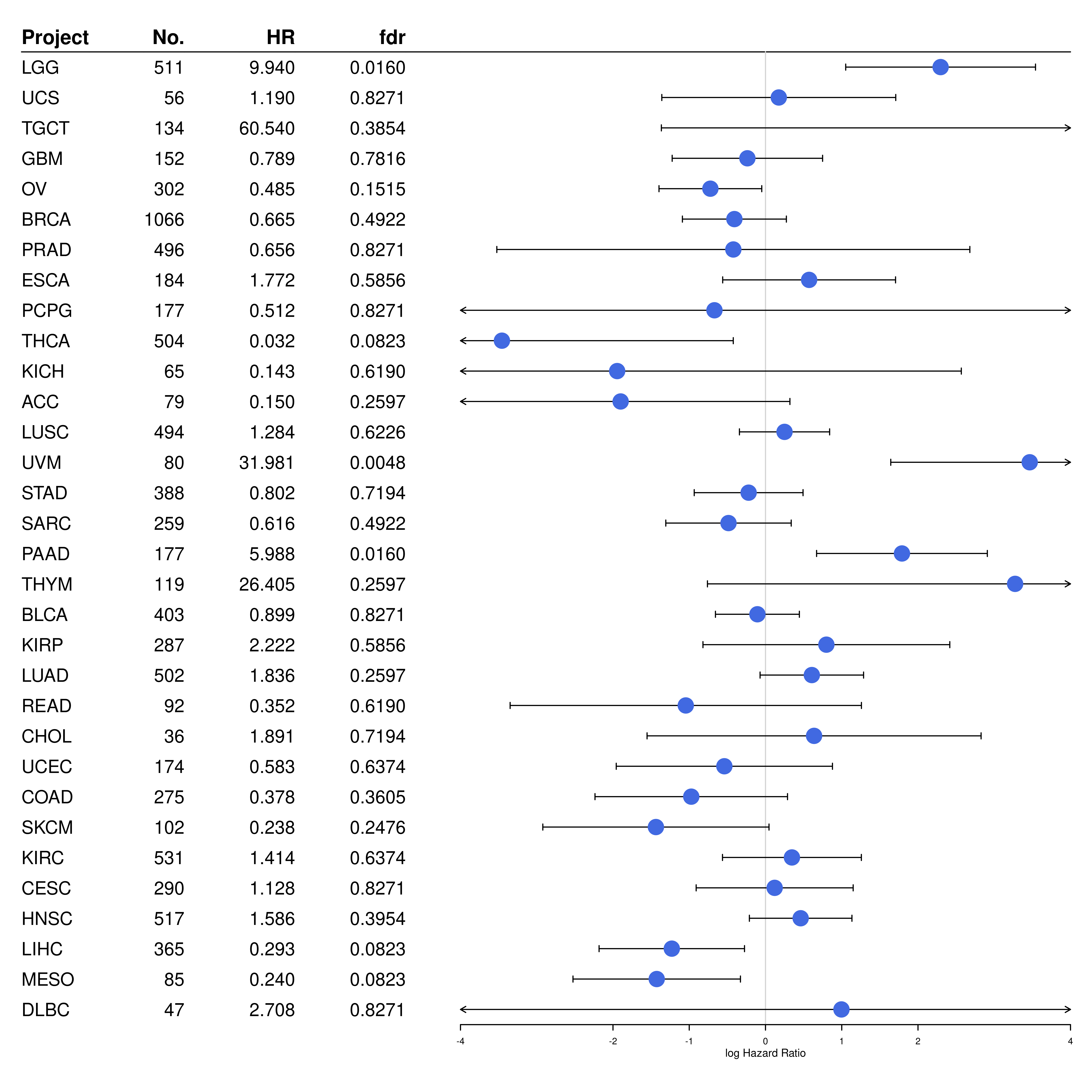
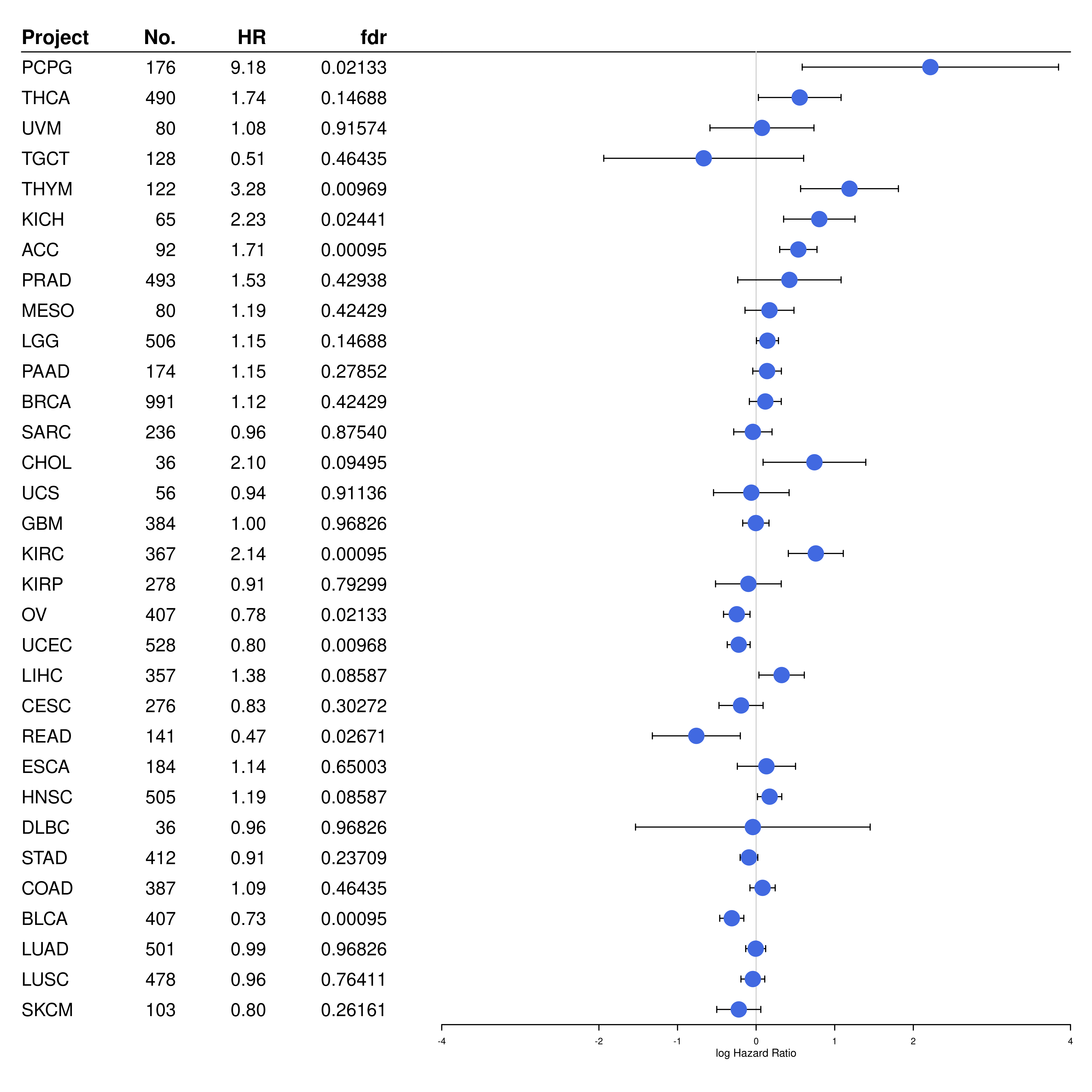
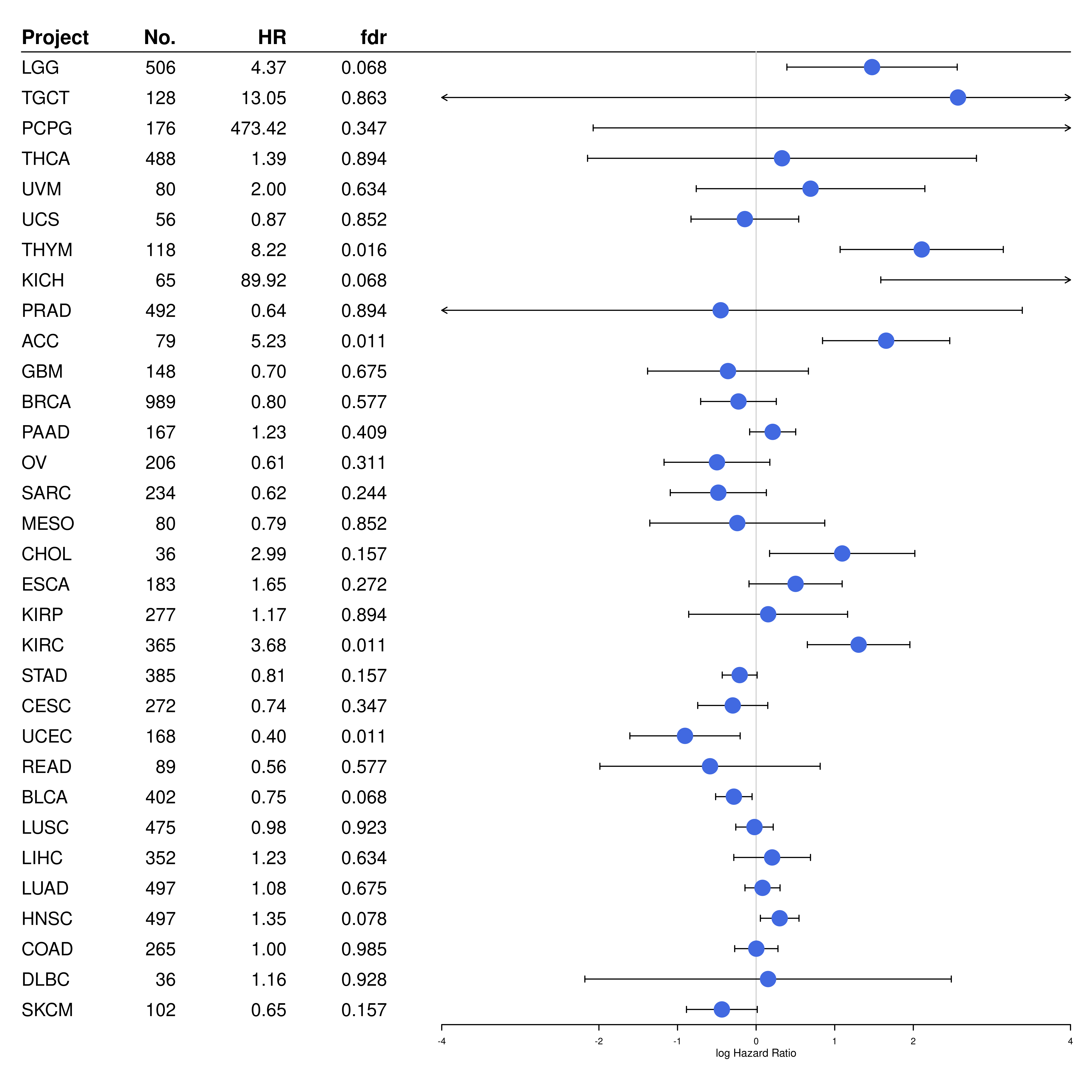
#> 3 TIGS 8413 1.34 1.27 1.42 2.49e-22We access survival effects of APS, TMB and TIGS across TCGA studies using unvariable cox model.
Firstly, we implement cox model and then obtain key result values from fit, i.e. p value and corresponding 95% confident interval.
library(survival)
# calculate APM cox model by project
model_APM <- df_os %>%
  filter(!is.na(nAPM)) %>%
  group_by(Project) %>%
  dplyr::do(coxfit = coxph(Surv(time = Time, event = Event) ~ nAPM, data = .)) %>%
  summarise(
    Project = Project,
    Coef = summary(coxfit)$conf.int[1],
    Lower = summary(coxfit)$conf.int[3],
    Upper = summary(coxfit)$conf.int[4],
    Pvalue = summary(coxfit)$logtest[3]
  )

# use nTMB or log(nTMB)
model_TMB <- df_os %>%
  filter(!is.na(nTMB)) %>%
  group_by(Project) %>%
  dplyr::do(coxfit = coxph(Surv(time = Time, event = Event) ~ log(nTMB), data = .)) %>%
  summarise(
    Project = Project,
    Coef = summary(coxfit)$conf.int[1],
    Lower = summary(coxfit)$conf.int[3],
    Upper = summary(coxfit)$conf.int[4],
    Pvalue = summary(coxfit)$logtest[3]
  )

model_TIGS <- df_os %>%
  filter(!is.na(TIGS)) %>%
  group_by(Project) %>%
  dplyr::do(coxfit = coxph(Surv(time = Time, event = Event) ~ TIGS, data = .)) %>%
  summarise(
    Project = Project,
    Coef = summary(coxfit)$conf.int[1],
    Lower = summary(coxfit)$conf.int[3],
    Upper = summary(coxfit)$conf.int[4],
    Pvalue = summary(coxfit)$logtest[3]
  )

N_APM <- df_os %>%
  filter(!is.na(nAPM)) %>%
  group_by(Project) %>%
  summarise(N = n())

N_TMB <- df_os %>%
  filter(!is.na(nTMB)) %>%
  group_by(Project) %>%
  summarise(N = n())

N_TIGS <- df_os %>%
  filter(!is.na(TIGS)) %>%
  group_by(Project) %>%
  summarise(N = n())


cox_APM <- full_join(model_APM, N_APM)
#> Joining, by = "Project"
cox_TMB <- full_join(model_TMB, N_TMB)
#> Joining, by = "Project"
cox_TIGS <- full_join(model_TIGS, N_TIGS)
#> Joining, by = "Project"


save(cox_APM, cox_TMB, cox_TIGS, df_summary, file = "results/unicox.RData")UPDATE: Adjust p values and order them by median APM/TMB/TIGS.
cox_APM <- cox_APM %>%
  mutate(Pvalue = p.adjust(Pvalue, method = "fdr")) %>%
  arrange(factor(Project, levels = arrange(df_summary, medianAPM) %>% .$Project))

cox_TMB <- cox_TMB %>%
  mutate(Pvalue = p.adjust(Pvalue, method = "fdr")) %>%
  arrange(factor(Project, levels = arrange(df_summary, medianTMB) %>% .$Project))

cox_TIGS <- cox_TIGS %>%
  mutate(Pvalue = p.adjust(Pvalue, method = "fdr")) %>%
  arrange(factor(Project, levels = arrange(df_summary, medianTIGS) %>% .$Project))
Secondly, we generate forest plot.
library(forestplot)
#> Loading required package: grid
#> Loading required package: checkmate

########### Forest plot

#------ APM
options(digits = 2)
forest_APM <- rbind(
  c("Project", NA, NA, NA, "fdr", "No."),
  cox_APM
) %>% as.data.frame()
forest_APM$HR <- c("HR", format(as.numeric(forest_APM$Coef[-1]), digits = 2))
forest_APM$Pvalue <- c("fdr", format(as.numeric(forest_APM$Pvalue[-1]), digits = 2))

forestplot(
  fn.ci_norm = fpDrawCircleCI,
  forest_APM[, c("Project", "N", "HR", "Pvalue")],
  mean = c(NA, log(cox_APM$Coef)), lower = c(NA, log(cox_APM$Lower)), upper = c(NA, log(cox_APM$Upper)),
  is.summary = c(TRUE, rep(FALSE, 32)),
  clip = c(-4, 4), zero = 0,
  col = fpColors(box = "royalblue", line = "black", summary = "royalblue", hrz_lines = "black"),
  vertices = TRUE,
  xticks = c(-4, -2, -1, 0, 1, 2, 4),
  hrzl_lines = list("2" = gpar(lty = 1, col = "black")),
  boxsize = 0.5,
  # graph.pos = 3,
  xlab = "log Hazard Ratio"
)
#pdf("forestplot_APS.pdf", onefile = F)
forestplot(
  fn.ci_norm = fpDrawCircleCI,
  forest_APM[, c("Project", "N", "HR", "Pvalue")],
  mean = c(NA, log(cox_APM$Coef)), lower = c(NA, log(cox_APM$Lower)), upper = c(NA, log(cox_APM$Upper)),
  is.summary = c(TRUE, rep(FALSE, 32)),
  clip = c(-4, 4), zero = 0,
  col = fpColors(box = "royalblue", line = "black", summary = "royalblue", hrz_lines = "black"),
  vertices = TRUE,
  xticks = c(-4, -2, -1, 0, 1, 2, 4),
  hrzl_lines = list("2" = gpar(lty = 1, col = "black")),
  boxsize = 0.5,
  # graph.pos = 3,
  xlab = "log Hazard Ratio"
)
#dev.off()

#----- TMB
forest_TMB <- rbind(
  c("Project", NA, NA, NA, "fdr", "No."),
  cox_TMB
) %>% as.data.frame()
forest_TMB$HR <- c("HR", format(as.numeric(forest_TMB$Coef[-1]), digits = 2))
forest_TMB$Pvalue <- c("fdr", format(as.numeric(forest_TMB$Pvalue[-1]), digits = 2))


#pdf("forestplot_TMB.pdf", onefile = F)
forestplot(
  fn.ci_norm = fpDrawCircleCI,
  forest_TMB[, c("Project", "N", "HR", "Pvalue")],
  mean = c(NA, log(cox_TMB$Coef)), lower = c(NA, log(cox_TMB$Lower)), upper = c(NA, log(cox_TMB$Upper)),
  is.summary = c(TRUE, rep(FALSE, 32)),
  clip = c(-4, 4), zero = 0,
  col = fpColors(box = "royalblue", line = "black", summary = "royalblue", hrz_lines = "black"),
  vertices = TRUE,
  xticks = c(-4, -2, -1, 0, 1, 2, 4),
  hrzl_lines = list("2" = gpar(lty = 1, col = "black")),
  boxsize = 0.5,
  # graph.pos = 3,
  xlab = "log Hazard Ratio"
)
#dev.off()

#---------- TIGS
forest_TIGS <- rbind(
  c("Project", NA, NA, NA, "fdr", "No."),
  cox_TIGS
) %>% as.data.frame()
forest_TIGS$HR <- c("HR", format(as.numeric(forest_TIGS$Coef[-1]), digits = 2))
forest_TIGS$Pvalue <- c("fdr", format(as.numeric(forest_TIGS$Pvalue[-1]), digits = 2))


#pdf("forestplot_TIGS.pdf", onefile = F)
forestplot(
  fn.ci_norm = fpDrawCircleCI,
  forest_TIGS[, c("Project", "N", "HR", "Pvalue")],
  mean = c(NA, log(cox_TIGS$Coef)), lower = c(NA, log(cox_TIGS$Lower)), upper = c(NA, log(cox_TIGS$Upper)),
  is.summary = c(TRUE, rep(FALSE, 32)),
  clip = c(-4, 4), zero = 0,
  col = fpColors(box = "royalblue", line = "black", summary = "royalblue", hrz_lines = "black"),
  vertices = TRUE,
  xticks = c(-4, -2, -1, 0, 1, 2, 4),
  hrzl_lines = list("2" = gpar(lty = 1, col = "black")),
  boxsize = 0.5,
  # graph.pos = 3,
  xlab = "log Hazard Ratio"
)
APS, TIGS and B2M mutation
Obtain B2M mutation status.
rm(list = ls())

# load package
require(TCGAmutations)


study_list <- tcga_available()$Study_Abbreviation[-34]
cohorts <- system.file("extdata", "cohorts.txt", package = "TCGAmutations")
cohorts <- data.table::fread(input = cohorts)

# calculate TMB
lapply(study_list, function(study) {
  require(maftools)
  TCGAmutations::tcga_load(study)
  maf <- eval(as.symbol(tolower(paste0("TCGA_", study, "_mc3"))))
  maf@data %>%
    group_by(Tumor_Sample_Barcode) %>%
    summarise(B2M = sum(grepl("^B2M$", Hugo_Symbol)))
}) -> tcga_b2m
names(tcga_b2m) <- study_list

# 33 study available, merge them
TCGA_B2M <- purrr::reduce(tcga_b2m, dplyr::bind_rows)

if (!file.exists("results/TCGA_B2M.RData")) {
  save(TCGA_B2M, file = "results/TCGA_B2M.RData")
}

rm(list = grep("tcga_*", ls(), value = TRUE))
rm(list = ls())rm(list = ls())
load(file = "results/TCGA_B2M.RData")
load(file = "results/TCGA_ALL.RData")
tcga_all <- tcga_all %>%
mutate(
nAPM = (APM - min(APM, na.rm = TRUE)) / (max(APM, na.rm = TRUE) - min(APM, na.rm = TRUE)),
nTMB = TMB_NonsynVariants / 38,
TIGS = log(nTMB + 1) * nAPM
)
df_b2m <-
dplyr::inner_join(tcga_all, TCGA_B2M, by = "Tumor_Sample_Barcode")
table(df_b2m$B2M)
#>
#> 0 1 2 3 4
#> 10007 92 27 4 1
df_b2m <- df_b2m %>%
dplyr::mutate(
B2M_Status = ifelse(B2M > 0, "Mutant", "WT")
) %>%
dplyr::filter(!is.na(APM), !is.na(TIGS), !is.na(B2M))ggpubr::ggboxplot(
df_b2m,
x = "B2M_Status", y = "APM",
ylab = "APS", xlab = "B2M mutation status"
) +
ggpubr::stat_compare_means(method = "t.test", label.x = 1.3)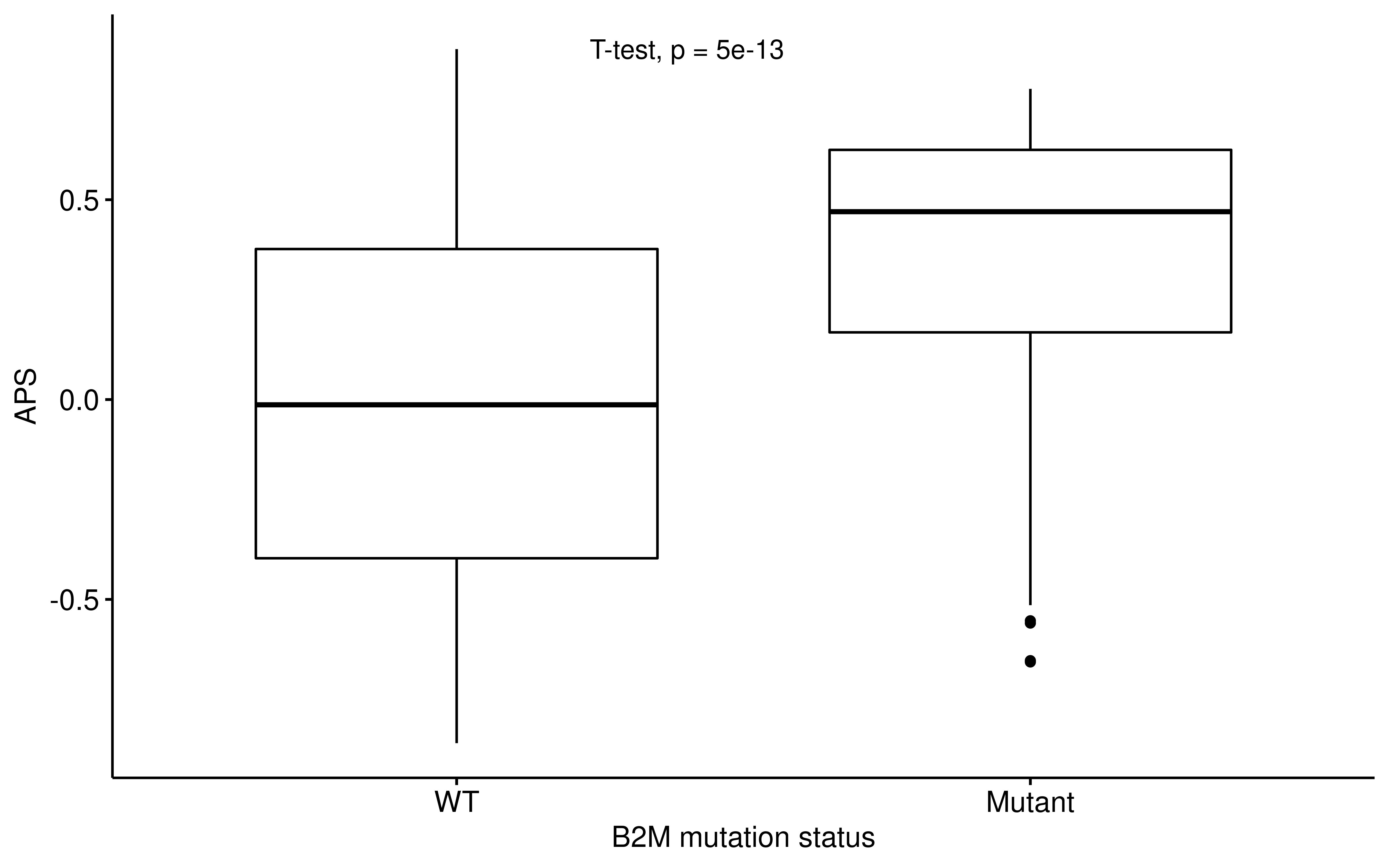
ggpubr::ggboxplot(
  df_b2m,
  x = "B2M_Status", y = "TIGS",
  xlab = "B2M mutation status"
) +
  ggpubr::stat_compare_means(method = "t.test", label.x = 1.3)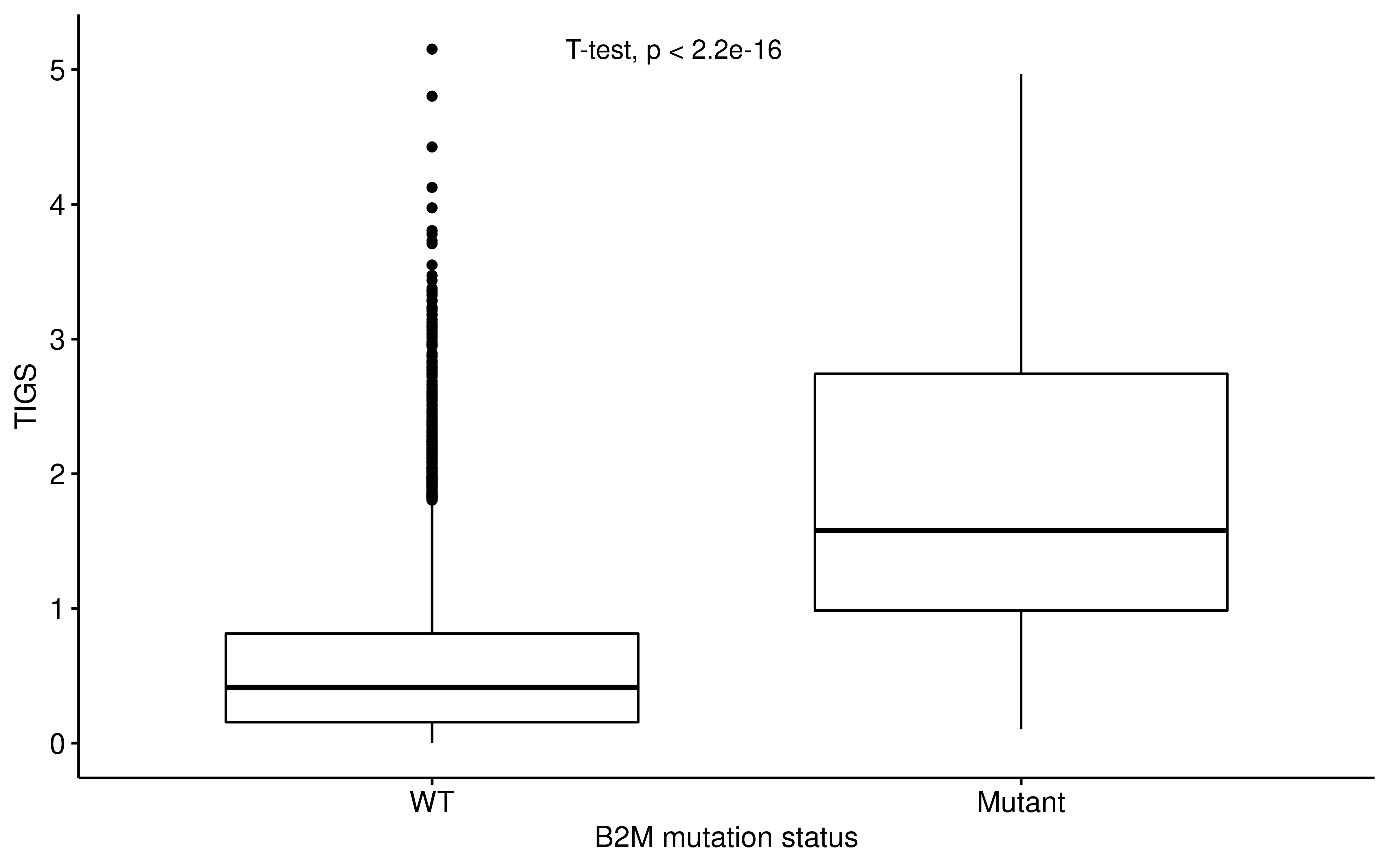
ggpubr::ggboxplot(
  df_b2m,
  x = "B2M_Status", y = "TMB_NonsynVariants",
  ylab = "TMB", xlab = "B2M mutation status"
) +
  ggpubr::stat_compare_means(method = "wilcox.test", label.x = 1.3)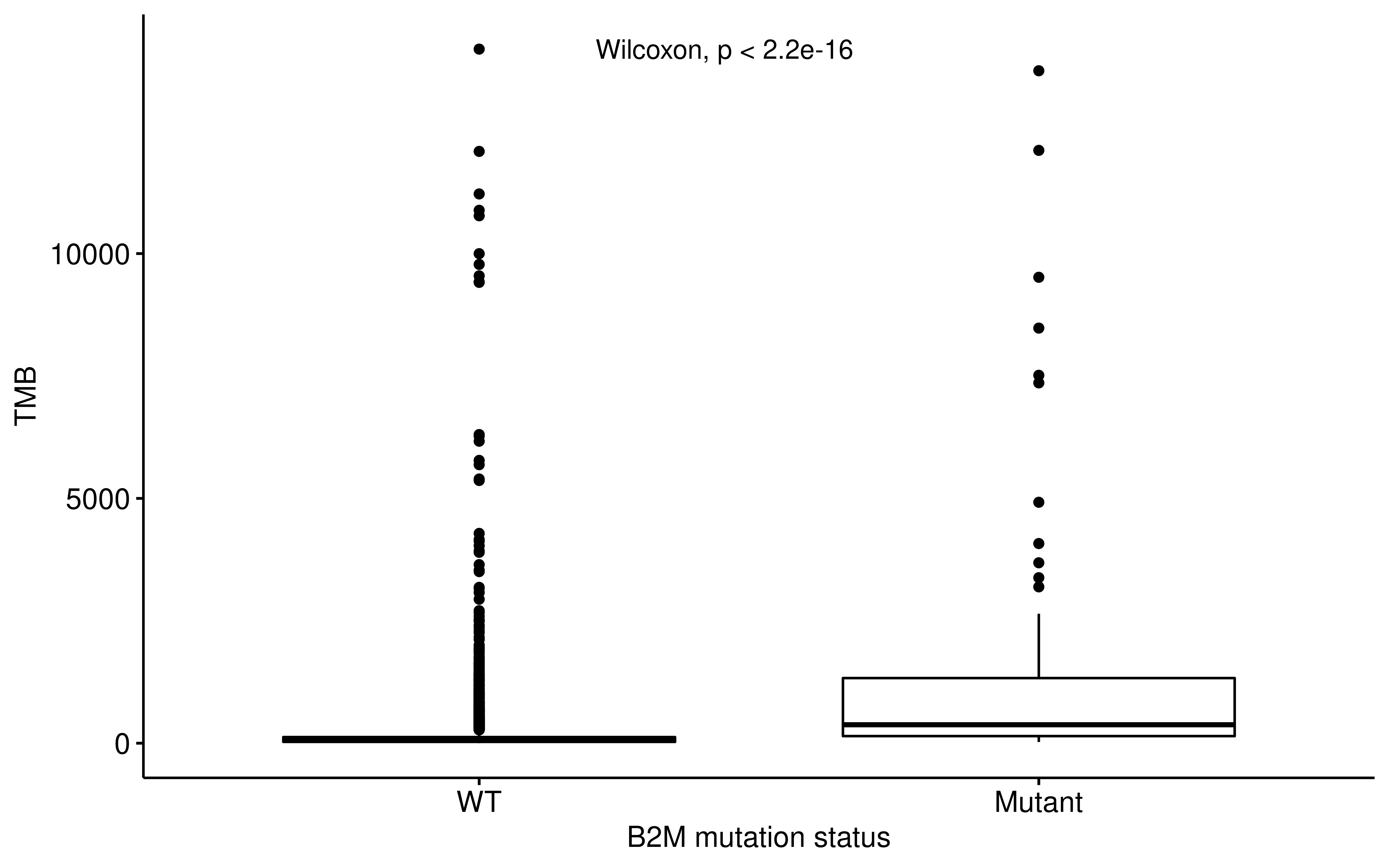
Focus on tructing mutation https://www.nejm.org/doi/10.1056/NEJMoa1604958?url_ver=Z39.88-2003&rfr_id=ori:rid:crossref.org&rfr_dat=cr_pub%3dwww.ncbi.nlm.nih.gov
rm(list = ls())

# load package
require(TCGAmutations)


study_list <- tcga_available()$Study_Abbreviation[-34]
cohorts <- system.file("extdata", "cohorts.txt", package = "TCGAmutations")
cohorts <- data.table::fread(input = cohorts)

# calculate TMB
lapply(study_list, function(study) {
  require(maftools)
  TCGAmutations::tcga_load(study)
  maf <- eval(as.symbol(tolower(paste0("TCGA_", study, "_mc3"))))
  rbind(maf@data, maf@maf.silent) %>%
    group_by(Tumor_Sample_Barcode) %>%
    summarise(B2M = sum(grepl("^B2M$", Hugo_Symbol)
    & Variant_Classification %in% c("Nonsense_Mutation")))
}) -> tcga_b2m
names(tcga_b2m) <- study_list

# 33 study available, merge them
TCGA_B2M <- purrr::reduce(tcga_b2m, dplyr::bind_rows)

if (!file.exists("results/TCGA_B2M2.RData")) {
  save(TCGA_B2M, file = "results/TCGA_B2M2.RData")
}

rm(list = grep("tcga_*", ls(), value = TRUE))
rm(list = ls())rm(list = ls())
load(file = "results/TCGA_B2M2.RData")
load(file = "results/TCGA_ALL.RData")
tcga_all <- tcga_all %>%
mutate(
nAPM = (APM - min(APM, na.rm = TRUE)) / (max(APM, na.rm = TRUE) - min(APM, na.rm = TRUE)),
nTMB = TMB_NonsynVariants / 38,
TIGS = log(nTMB + 1) * nAPM
)
df_b2m <-
dplyr::inner_join(tcga_all, TCGA_B2M, by = "Tumor_Sample_Barcode")
table(df_b2m$B2M)
#>
#> 0 1 2
#> 10129 15 3
df_b2m <- df_b2m %>%
dplyr::mutate(
B2M_Status = ifelse(B2M > 0, "Nonsense", "Non-nonsense")
) %>%
dplyr::filter(!is.na(APM), !is.na(TIGS), !is.na(B2M))ggpubr::ggboxplot(
df_b2m,
x = "B2M_Status", y = "APM",
ylab = "APS", xlab = "B2M mutation status"
) +
ggpubr::stat_compare_means(method = "t.test", label.x = 1.3)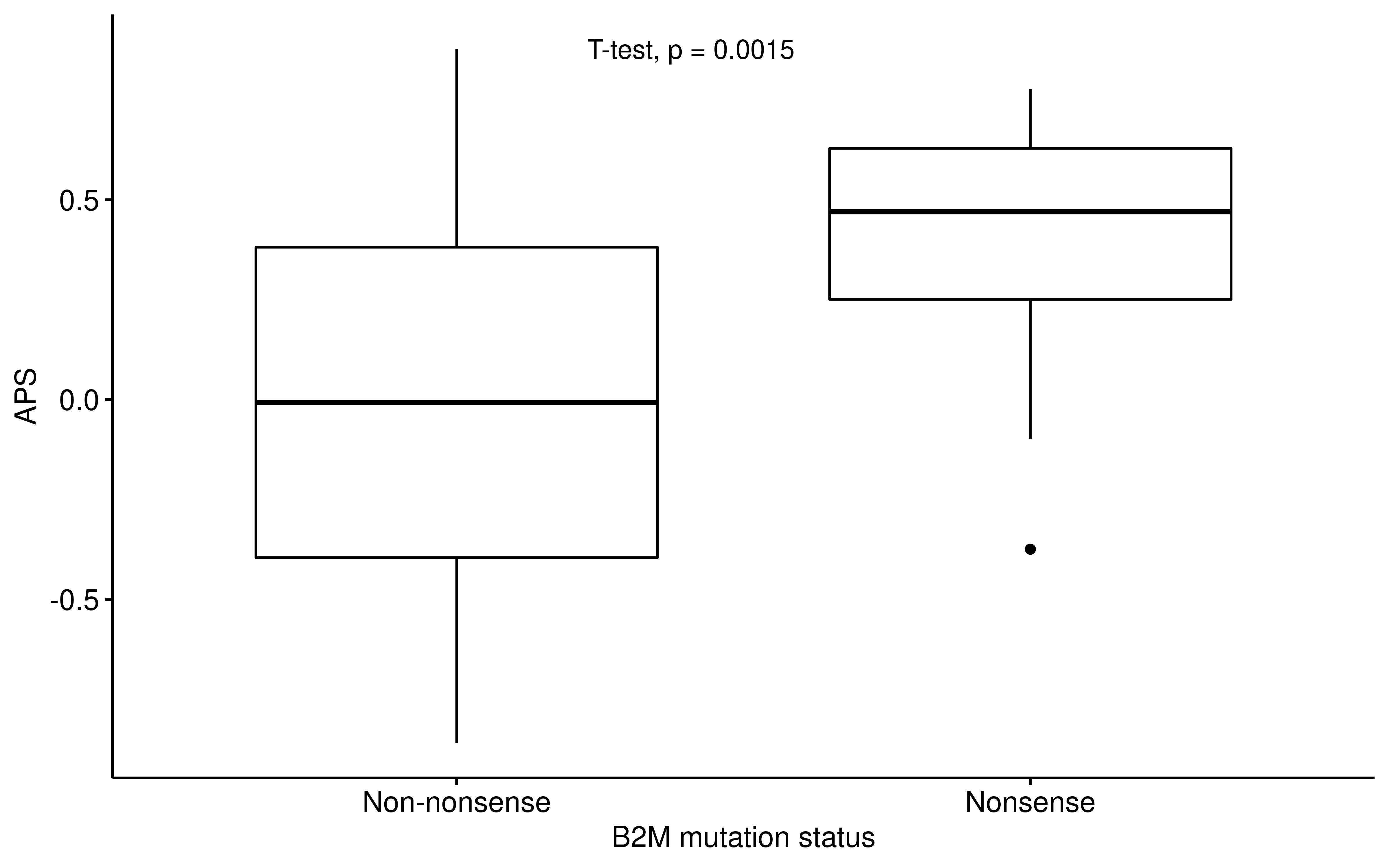
ggpubr::ggboxplot(
  df_b2m,
  x = "B2M_Status", y = "TIGS",
  xlab = "B2M mutation status"
) +
  ggpubr::stat_compare_means(method = "t.test", label.x = 1.3)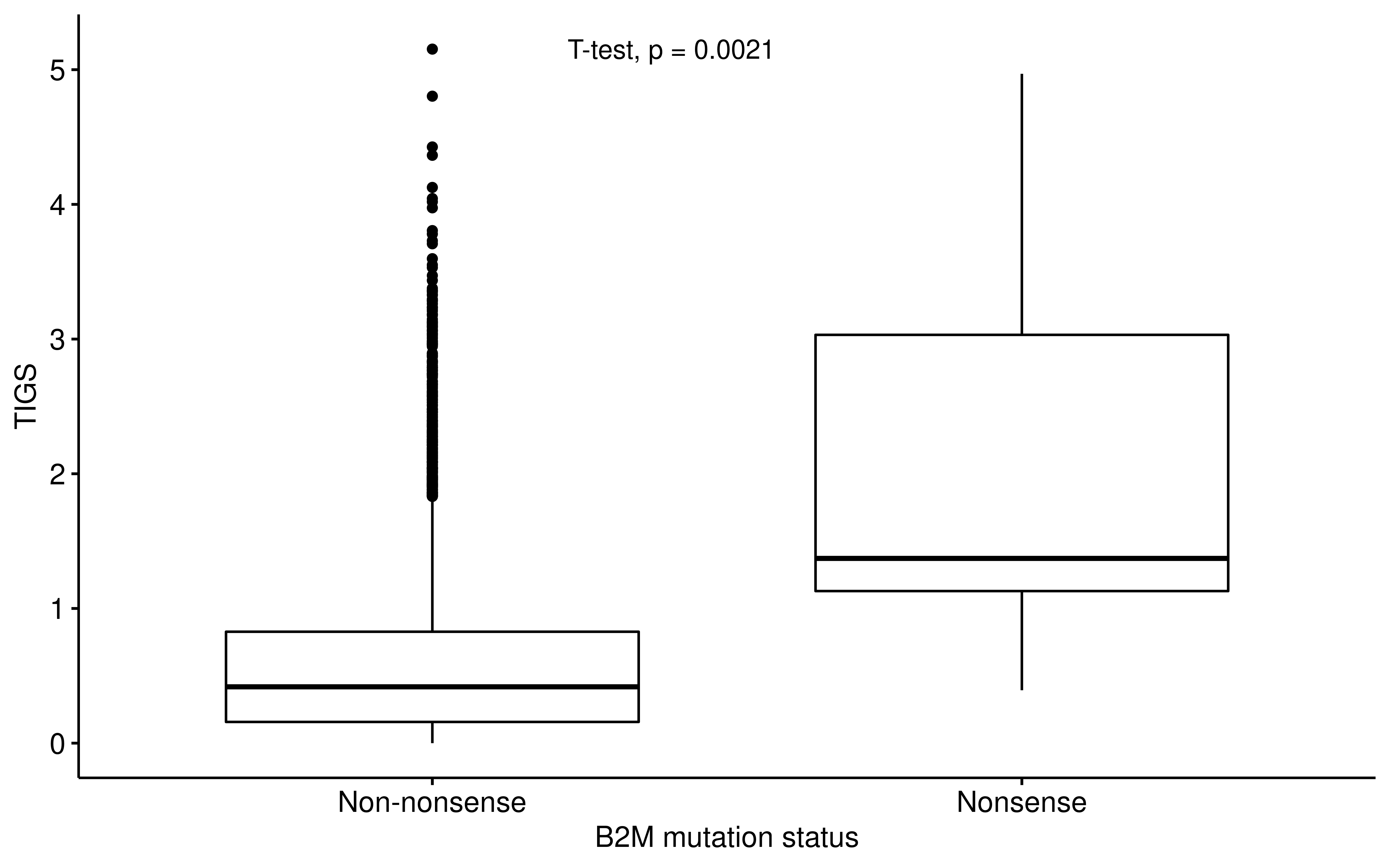
ggpubr::ggboxplot(
  df_b2m,
  x = "B2M_Status", y = "TMB_NonsynVariants",
  ylab = "TMB", xlab = "B2M mutation status"
) +
  ggpubr::stat_compare_means(method = "wilcox.test", label.x = 1.3)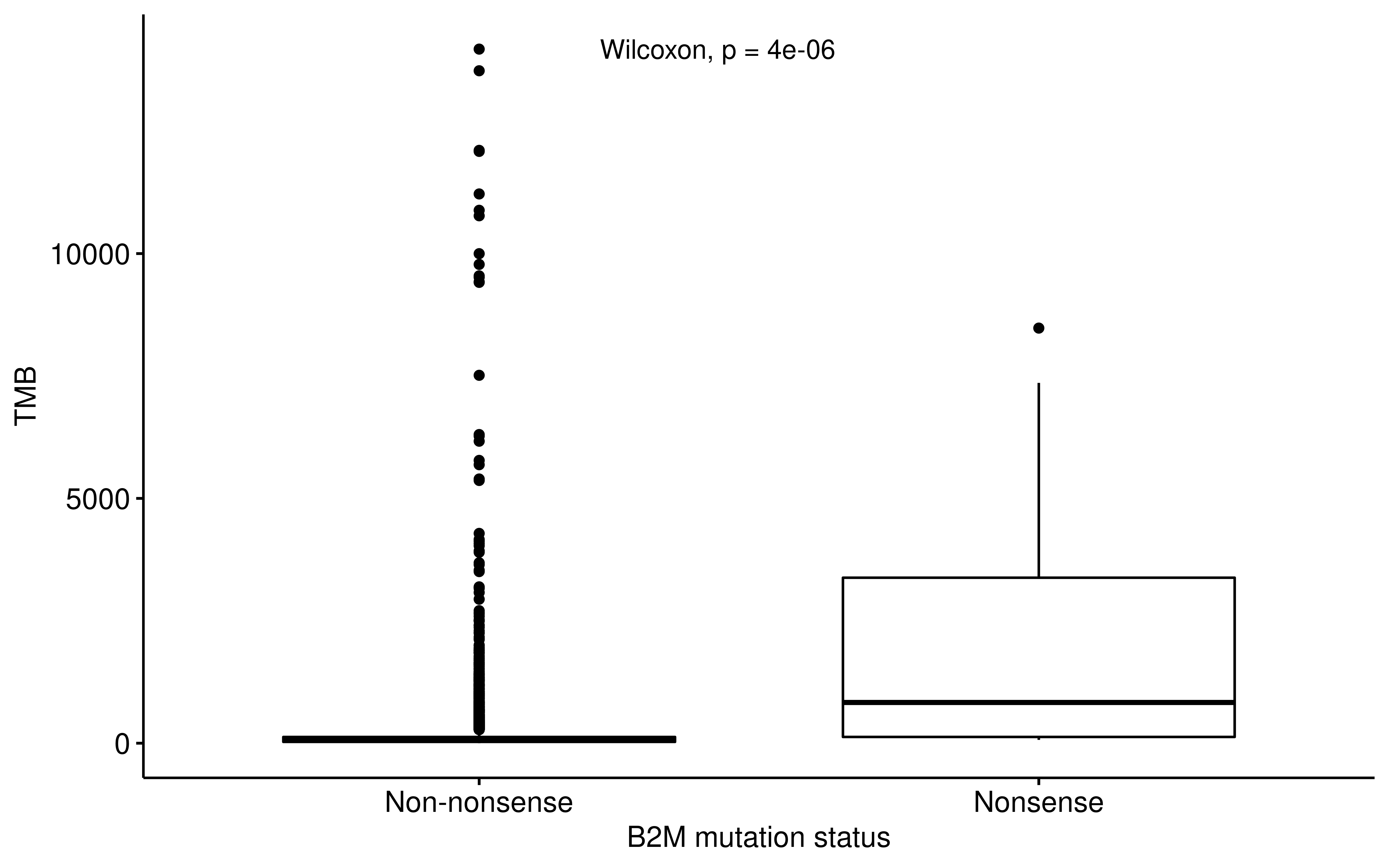
Check gene expression in these mutant samples.
load("results/TCGA_RNASeq_PanCancer.RData")
B2M_expr <- RNASeq_pancan %>%
  dplyr::filter(sample == "B2M") %>%
  dplyr::select(-sample) %>%
  as.numeric()

B2M_expr <- dplyr::tibble(
  Tumor_Sample_Barcode = colnames(RNASeq_pancan)[-1],
  B2M_expr = B2M_expr
) %>%
  dplyr::filter(substr(Tumor_Sample_Barcode, 14, 15) == "01") %>%
dplyr::mutate(Tumor_Sample_Barcode = substr(Tumor_Sample_Barcode, 1, 12))ggpubr::ggboxplot(
B2M_expr,
x = "B2M_Status", y = "B2M_expr",
xlab = "B2M mutation status"
) +
ggpubr::stat_compare_means(method = "t.test", label.x = 1.3)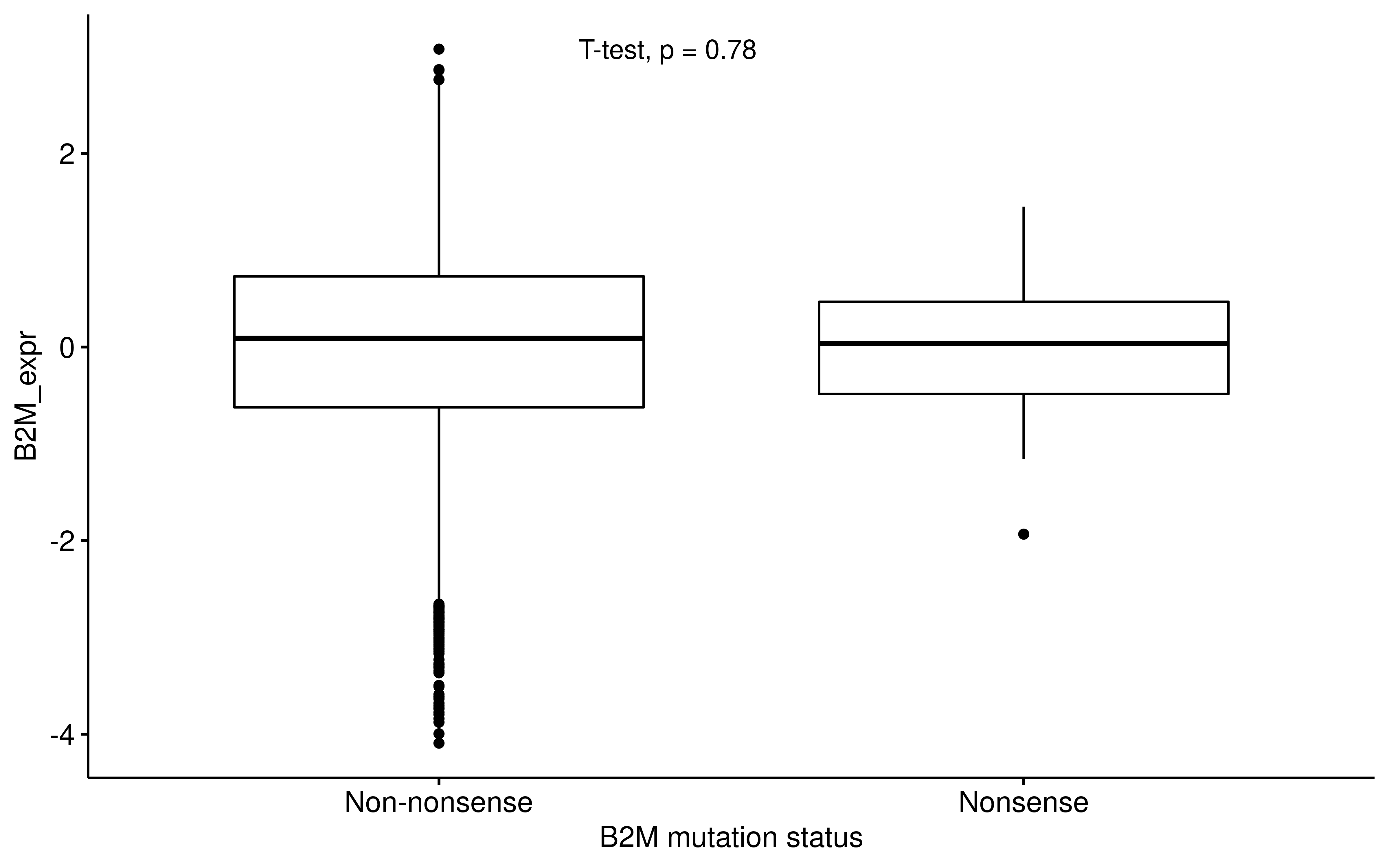
Therefore, APS/TIGS cannot capture whether B2M lose function or not. However, we do observe that B2M mutation upgrade APS/TIGS, this may be explained by compensatory expression of APS gene signature.
Gene sets enriched in patients with high APM score
To identify the specific gene sets/pathway associated with high APS, we firstly run differential gene expression analysis for each TCGA cancer type based on APS status. Patients with APS of first quartile was defined as “APS-High”, patients with APS of the forth quartile was defined as “APS-Low”. Genes with p value <0.01 and FDR <0.05 were ranked by logFC from top to bottom and then inputted into GSEA function of R package clusterProfiler with custom gene sets download from Molecular Signature Database v6.2. Normalized enrichment score (NES) was used to rank the differentially enriched gene sets. In results from hallmark gene sets, several gene signatures (especially interferon alpha/gamma response) were found to be enriched in most TCGA cancer types with high APS, suggesting high APS are strongly associated with interferon alpha/gamma signaling pathway.
The code below is runned on linux server (need much time), thus if reader wanna reproduce it, you may need to download gene sets from Molecular Signature Database v6.2 and modify some file path.
rm(list = ls())
#----------------------------------------
# APM DEG and Pathway Enrichment Analysis
#----------------------------------------
library(tidyverse)

load("results/TCGA_RNASeq_PanCancer.RData")
load("results/gsva_tcga_pancan.RData")
load("results/TCGA_tidy_Clinical.RData")

df.gsva <- full_join(TCGA_Clinical.tidy, gsva.pac, by = c("Tumor_Sample_Barcode" = "tsb"))

tcga_info <- df.gsva
rm(df.gsea, df.gsva)
gc()

tcga_info <- tcga_info %>%
  select(Project:OS.time, Age, Gender, sample_type, Tumor_stage, APM) %>%
  filter(!is.na(APM))

projects <- unique(tcga_info[, "Project"])
samples <- colnames(RNASeq_pancan)[-1]

#-----------------------------------
# Build a workflow to calculate DEGs
#-----------------------------------
findDEGs <- function(info_df = NULL, expr_df = NULL, col_sample = "Tumor_Sample_Barcode", col_group = "APM",
                     col_subset = "Project", method = "limma", threshold = 0.25,
                     save = FALSE, filename = NULL) {
  stopifnot(!is.null(info_df), !is.null(expr_df))
  stopifnot(threshold >= 0 & threshold <= 1)

  if (!require(data.table)) {
    install.packages("data.table", dependencies = TRUE)
  }

  info_df <- setDT(info_df[, c(col_sample, col_group, col_subset)])
  colnames(info_df) <- c("sample", "groupV", "subset")
  info_df <- info_df[sample %in% colnames(expr_df)]
  info_df <- info_df[!is.na(subset)]
  all_sets <- unique(info_df[, subset])


  if ("DEGroup" %in% colnames(info_df)) {
    stop("DEGroup column exists, please rename and re-run.")
  }

  # set threshold
  th1 <- threshold
  th2 <- 1 - th1

  info_df[, DEGroup := ifelse(groupV < quantile(groupV, th1), "Low",
    ifelse(groupV > quantile(groupV, th2), "High", NA)
  ), by = subset]
  info_df <- info_df[!is.na(DEGroup)]
  sets <- unique(info_df[, subset])
  may_del <- setdiff(all_sets, sets)
  if (length(may_del) != 0) {
    message("Following groups has been filtered out because of threshold setting, you better check")
    print(may_del)
  }

  info_list <- lapply(sets, function(x) info_df[subset == x])
  names(info_list) <- sets

  col1 <- colnames(expr_df)[1]


  options(digits = 4)

  doDEG <- function(input, method = NULL) {
    #-- prepare
    exprSet <- expr_df[, c(col1, input$sample)]
    exprSet <- as.data.frame(exprSet)
    exprSet <- na.omit(exprSet)
    input <- as.data.frame(input)
    rownames(exprSet) <- exprSet[, 1]
    exprSet <- exprSet[, -1]

    sample_tb <- table(input$DEGroup)

    #--- make sure have some samples
    if (!length(sample_tb) < 2 & all(sample_tb >= 5)) {
      group_list <- input$DEGroup

      if ("limma" %in% method) {
        suppressMessages(library(limma))
        design <- model.matrix(~ 0 + factor(group_list))
        colnames(design) <- c("High", "Low")
        cont.matrix <- makeContrasts("High-Low", levels = design)

        fit <- lmFit(exprSet, design)
        fit2 <- contrasts.fit(fit, cont.matrix)
        fit2 <- eBayes(fit2)
        topTable(fit2, number = Inf, adjust.method = "BH")
      }
    }
  }

  res <- lapply(info_list, doDEG, method = method)
  names(res) <- sets
  return(res)
}

# threshold = 0.25 is used in manuscript
# DEG_pancan2 = findDEGs(info_df = tcga_info, expr_df = RNASeq_pancan)
# Here we use threshold = 0.5 to do this analysis to respond
# reviewer's comment
DEG_pancan2 <- findDEGs(info_df = tcga_info, expr_df = RNASeq_pancan, threshold = 0.5)
save(DEG_pancan2, file = "results/DEG_pancan.RData")

#----------------------------------------------------
# Pathway enrichment analysis using clusterProfiler
#--------------------------------------------------
load(file = "results/DEG_pancan.RData")
library(clusterProfiler)
library(tidyverse)
library(openxlsx)

#---------------

## - setting
pvalue <- 0.01
adj.pvalue <- 0.05

## - process

#------- Reading GSEA genesets files
hallmark <- read.gmt("/public/data/VM_backup/biodata/MsigDB/h.all.v6.2.symbols.gmt")
c1 <- read.gmt("/public/data/VM_backup/biodata/MsigDB/c1.all.v6.2.symbols.gmt")
c2_kegg <- read.gmt("/public/data/VM_backup/biodata/MsigDB/c2.cp.kegg.v6.2.symbols.gmt")
c2_reactome <- read.gmt("/public/data/VM_backup/biodata/MsigDB/c2.cp.reactome.v6.2.symbols.gmt")
c3 <- read.gmt("/public/data/VM_backup/biodata/MsigDB/c3.all.v6.2.symbols.gmt")
c4 <- read.gmt("/public/data/VM_backup/biodata/MsigDB/c4.all.v6.2.symbols.gmt")
c5_mf <- read.gmt("/public/data/VM_backup/biodata/MsigDB/c5.mf.v6.2.symbols.gmt")
c5_bp <- read.gmt("/public/data/VM_backup/biodata/MsigDB/c5.bp.v6.2.symbols.gmt")
c6 <- read.gmt("/public/data/VM_backup/biodata/MsigDB/c6.all.v6.2.symbols.gmt")
c7 <- read.gmt("/public/data/VM_backup/biodata/MsigDB/c7.all.v6.2.symbols.gmt")
#-=---------

goGSEA <- function(DEG, prefix = NULL, pvalue = 0.01, adj.pvalue = 0.05, destdir = "~/projects/tumor-immunogenicity-score/report/results/GSEA_results") {
  library(clusterProfiler)
  library(openxlsx)
  library(tidyverse)

  filterDEG <- subset(DEG, subset = P.Value < pvalue & adj.P.Val < adj.pvalue)
  filterDEG$SYMBOL <- rownames(filterDEG)
  filterDEG <- filterDEG %>%
    arrange(desc(logFC), adj.P.Val)
  geneList <- filterDEG$logFC
  names(geneList) <- filterDEG$SYMBOL

  res <- list()
  if (base::exists("hallmark")) res$hallmark <- GSEA(geneList, TERM2GENE = hallmark, verbose = FALSE)
  # if (base::exists("c1")) res$c1 = GSEA(geneList, TERM2GENE=c1, verbose=FALSE)
  if (base::exists("c2_kegg")) res$c2_kegg <- GSEA(geneList, TERM2GENE = c2_kegg, verbose = FALSE)
  if (base::exists("c2_reactome")) res$c2_reactome <- GSEA(geneList, TERM2GENE = c2_reactome, verbose = FALSE)
  # if (base::exists("c3")) res$c3 = GSEA(geneList, TERM2GENE=c3, verbose=FALSE)
  # if (base::exists("c4")) res$c4 = GSEA(geneList, TERM2GENE=c4, verbose=FALSE)
  if (base::exists("c5_mf")) res$c5_mf <- GSEA(geneList, TERM2GENE = c5_mf, verbose = FALSE)
  if (base::exists("c5_bp")) res$c5_bp <- GSEA(geneList, TERM2GENE = c5_bp, verbose = FALSE)
  if (base::exists("c6")) res$c6 <- GSEA(geneList, TERM2GENE = c6, verbose = FALSE)
  if (base::exists("c7")) res$c7 <- GSEA(geneList, TERM2GENE = c7, verbose = FALSE)

  getResultList <- lapply(res, function(x) x@result)
  if (!dir.exists(destdir)) dir.create(destdir)
  outpath <- file.path(destdir, prefix)
  write.xlsx(x = getResultList, file = paste0(outpath, ".xlsx"))
  return(res)
}


# remove STAD, CHOL, KICH and DLBC
DEG_pancan2 <- DEG_pancan2[setdiff(names(DEG_pancan2), c("STAD", "CHOL", "KICH", "DLBC"))]
GSEA_list <- Map(goGSEA, DEG_pancan2, names(DEG_pancan2))
save(GSEA_list, file = "results/GSEA_results_rm_notEnriched.RData")

#------- GSEA example plot
# load("results/GSEA_results.RData")
load("results/GSEA_results_rm_notEnriched.RData")
library(clusterProfiler)

gseaplot(GSEA_list$SKCM$hallmark, geneSetID = "HALLMARK_INTERFERON_GAMMA_RESPONSE")

# gseaplot(egmt2, geneSetID = "INTEGRAL_TO_PLASMA_MEMBRANE")
# gseaplot(res$hallmark, geneSetID = "HALLMARK_INTERFERON_GAMMA_RESPONSE")

#------ get main result cloumn
gsea_results <- lapply(GSEA_list, function(x) {
  # x@result %>% select()
  lapply(x, function(gsea) {
    gsea@result %>% dplyr::select(ID, setSize, enrichmentScore, NES, pvalue, qvalues)
  })
})

save(gsea_results, file = "results/GSEA_results_notEnriched_small.RData")
rm(GSEA_list)
gc()

#----- plot
summariseGSEA <- function(pathway = NULL) {
  purrr::reduce(Map(function(x, y, pathway) {
    if (nrow(x[[pathway]]) == 0) {
      res <- NULL
    } else {
      res <- x[[pathway]]
      res$Project <- y
    }
    res
  }, gsea_results, names(gsea_results), pathway), rbind)
}

gsea_summary <- list()
gsea_summary$hallmark <- summariseGSEA(pathway = "hallmark")
# gsea_summary$c2_kegg = summariseGSEA(pathway = "c2_kegg")
gsea_summary$c2_reactome <- summariseGSEA(pathway = "c2_reactome")
gsea_summary$c5_mf <- summariseGSEA(pathway = "c5_mf")
gsea_summary$c5_bp <- summariseGSEA(pathway = "c5_bp")
gsea_summary$c6 <- summariseGSEA(pathway = "c6")
gsea_summary$c7 <- summariseGSEA(pathway = "c7")

save(gsea_summary, file = "results/GSEA_summary_notEnriched.RData")

## plot really
load("../data/df_combine_gsva_clinical.RData")

df.gsva %>%
  filter(!is.na(APM)) %>%
  group_by(Project) %>%
  summarize(MedianAPM = median(APM), N = n()) %>%
  arrange(MedianAPM) -> sortAPM
sortAPM %>% filter(Project != "DLBC") -> sortAPM

library(scales)
gsea_summary$hallmark %>%
  ggplot(mapping = aes(x = Project, y = ID)) +
  geom_tile(aes(fill = NES)) +
  scale_fill_gradient2(low = "blue", mid = "white", high = "red") +
  scale_x_discrete(limits = sortAPM$Project) + theme_classic() +
  theme(axis.text.x = element_text(angle = 30, hjust = 1, vjust = 1))

# df_wide = reshape2::dcast(gsea_summary$hallmark, ID ~ Project, value.var="NES", fill = 0)

library(pheatmap)

plotPathway <- function(df, save = FALSE, path = NULL, silent = FALSE) {
  df_wide <- reshape2::dcast(df, ID ~ Project, value.var = "NES", fill = 0)

  breaksList <- seq(-max(df_wide[, -1], na.rm = TRUE), max(df_wide[, -1], na.rm = TRUE), by = 0.01)
  pheatmap(df_wide %>% column_to_rownames(var = "ID"),
    color = colorRampPalette(c("blue", "white", "red"))(length(breaksList)),
    breaks = breaksList,
    # annotation_col = annotation_col,
    fontsize_row = 8, fontsize_col = 8, silent = silent,
    cellheight = 10, cellwidth = 10, filename = ifelse(save == FALSE, NA, path)
  )
}

gg <- plotPathway(gsea_summary$hallmark, silent = F, path = "results/GSEA_results_plot/Hallmark_Enriched.pdf", save = TRUE)
# gg = plotPathway(gsea_summary$c2_kegg, silent = F, path = "results/GSEA_results_plot/KEGG_Enriched.pdf", save = TRUE)
gg <- plotPathway(gsea_summary$c2_reactome, silent = F, path = "results/GSEA_results_plot/Reactome_Enriched.pdf", save = TRUE)
gg <- plotPathway(gsea_summary$c5_mf, silent = F, path = "results/GSEA_results_plot/GO_MolecuFunction_Enriched.pdf", save = TRUE)
gg <- plotPathway(gsea_summary$c5_bp, silent = F, path = "results/GSEA_results_plot/GO_BiologicalProcess_Enriched.pdf", save = TRUE)
gg <- plotPathway(gsea_summary$c6, silent = F, path = "results/GSEA_results_plot/C6_oncogenicsignatures_Enriched.pdf", save = TRUE)
gg <- plotPathway(gsea_summary$c7, silent = F, path = "results/GSEA_results_plot/C7_immunologicsignatures_Enriched.pdf", save = TRUE)

# gg


# _-------- rank pheatmap by NES value
plotPathway2 <- function(df, save = FALSE, path = NULL, silent = FALSE) {
  df_wide <- reshape2::dcast(df, ID ~ Project, value.var = "NES", fill = 0)
  df_wide <- df_wide[order(rowMeans(df_wide[, -1]), decreasing = TRUE), ]
  rownames(df_wide) <- NULL

  breaksList <- seq(-max(df_wide[, -1], na.rm = TRUE), max(df_wide[, -1], na.rm = TRUE), by = 0.01)

  pheatmap(df_wide %>% column_to_rownames(var = "ID"),
    color = colorRampPalette(c("blue", "white", "red"))(length(breaksList)),
    breaks = breaksList, cluster_rows = FALSE,
    # annotation_col = annotation_col,
    fontsize_row = 8, fontsize_col = 8, silent = silent,
    cellheight = 10, cellwidth = 10, filename = ifelse(save == FALSE, NA, path)
  )
}

gg <- plotPathway2(gsea_summary$c2_reactome, silent = F, path = "results/GSEA_results_plot/Reactome_Enriched2.pdf", save = TRUE)
Session Info
sessionInfo()
#> R version 3.6.0 (2019-04-26)
#> Platform: x86_64-pc-linux-gnu (64-bit)
#> Running under: CentOS Linux 7 (Core)
#>
#> Matrix products: default
#> BLAS:   /home/public/R/R-base/lib64/R/lib/libRblas.so
#> LAPACK: /home/public/R/R-base/lib64/R/lib/libRlapack.so
#>
#> locale:
#>  [1] LC_CTYPE=en_US.UTF-8       LC_NUMERIC=C
#>  [3] LC_TIME=en_US.UTF-8        LC_COLLATE=en_US.UTF-8
#>  [5] LC_MONETARY=en_US.UTF-8    LC_MESSAGES=en_US.UTF-8
#>  [7] LC_PAPER=en_US.UTF-8       LC_NAME=C
#>  [9] LC_ADDRESS=C               LC_TELEPHONE=C
#> [11] LC_MEASUREMENT=en_US.UTF-8 LC_IDENTIFICATION=C
#>
#> attached base packages:
#> [1] grid      stats     graphics  grDevices utils     datasets  methods
#> [8] base
#>
#> other attached packages:
#>  [1] forestplot_1.9      checkmate_1.9.4     survival_3.1-7
#>  [4] ggpubr_0.2.3        magrittr_1.5        scales_1.0.0
#>  [7] corrplot_0.84       pheatmap_1.0.12     forcats_0.4.0
#> [10] stringr_1.4.0       purrr_0.3.3         tidyr_1.0.0
#> [13] tibble_2.1.3        ggplot2_3.2.1       tidyverse_1.2.1
#> [16] readr_1.3.1         dplyr_0.8.3         UCSCXenaTools_1.2.7
#> [19] rmdformats_0.3.5    knitr_1.26          pacman_0.5.1
#>
#> loaded via a namespace (and not attached):
#>  [1] utf8_1.1.4             questionr_0.7.0        R.utils_2.9.0
#>  [4] tidyselect_0.2.5       lme4_1.1-21            robust_0.4-18.1
#>  [7] htmlwidgets_1.5.1      munsell_0.5.0          codetools_0.2-16
#> [10] DT_0.10                future_1.15.0          miniUI_0.1.1.1
#> [13] withr_2.1.2            Brobdingnag_1.2-6      metaBMA_0.6.2
#> [16] colorspace_1.4-1       highr_0.8              rstudioapi_0.10
#> [19] stats4_3.6.0           DescTools_0.99.30      robustbase_0.93-5
#> [22] rcompanion_2.3.7       ggsignif_0.6.0         listenv_0.7.0
#> [25] labeling_0.3           emmeans_1.4.2          rstan_2.19.2
#> [28] mnormt_1.5-5           MCMCpack_1.4-4         bridgesampling_0.7-2
#> [31] coda_0.19-3            vctrs_0.2.0            generics_0.0.2
#> [34] TH.data_1.0-10         metafor_2.1-0          xfun_0.11
#> [37] R6_2.4.0               BayesFactor_0.9.12-4.2 reshape_0.8.8
#> [40] logspline_2.1.15       assertthat_0.2.1       promises_1.1.0
#> [43] multcomp_1.4-10        ggExtra_0.9            gtable_0.3.0
#> [46] multcompView_0.1-7     globals_0.12.4         processx_3.4.1
#> [49] mcmc_0.9-6             sandwich_2.5-1         rlang_0.4.1
#> [52] MatrixModels_0.4-1     EMT_1.1                zeallot_0.1.0
#> [55] splines_3.6.0          TMB_1.7.15             lazyeval_0.2.2
#> [58] broom_0.5.2            inline_0.3.15          abind_1.4-5
#> [61] yaml_2.2.0             reshape2_1.4.3         modelr_0.1.5
#> [64] crosstalk_1.0.0        backports_1.1.5        httpuv_1.5.2
#> [67] tools_3.6.0            bookdown_0.15          psych_1.8.12
#> [70] ellipsis_0.3.0         RColorBrewer_1.1-2     WRS2_1.0-0
#> [73] ez_4.4-0               Rcpp_1.0.3             plyr_1.8.4
#>  [ reached getOption("max.print") -- omitted 98 entries ]
Immunotherapy datasets analyses
This part will clearly describe how to analyze APS, TMB and TIGS in immunotherapy datasets, including cancer type level and individual level. Raw data used for these analyses have been preprocessed, detail please read preprocessing part or TCGA pan-cancer analyses of this analysis report.
TIGS and pan-cancer objective response rate to PD-1 inhibition
Previous study has shown that TMB could predict pan-cancer ICI objective response rates (ORR). Here we will evaluate and compare the predictive power of APS, TIGS with TMB in pan-cancer ICI objective response rates prediction. The ORR for anti–PD-1 or anti–PD-L1 therapy will be plotted against the corresponding median APS, TIGS, TMB across multiple cancer types.
Through an extensive literature search, we identified 26 tumor types or subtypes for which data regarding the ORR are available. For each tumor type, we pooled the response data from the largest published studies that evaluated the ORR. We included only studies of anti–PD-1 or anti–PD-L1 monotherapy that enrolled at least 10 patients who were not selected for PD-L1 tumor expression (Identified individual studies and references are available in the manuscript Supplementary Table 3). The median tumor mutational burden for each tumor type was obtained from a validated comprehensive genomic profiling assay performed and provided by Foundation Medicine. The APS information for 23 tumor types were calculated based on TCGA datasets, and the APS for merkel cell carcinoma, cutaneous squamous cell carcinoma and small-cell lung cancer were calculated based on GEO microarray datasets.
Combination of datasets
In code implementation, we firstly combine APM score, TIGS score from TCGA studies and GEO datasets.
library(tidyverse)
## retrieve APM score
load("results/Add_gsva_scc_sclc_merkel.RData")

buildDF <- function(x, tumor_type = NULL) {
  stopifnot(!is.null(tumor_type))
  res <- x %>%
    dplyr::mutate(Project = tumor_type) %>%
    as.data.frame()
  res
}

lapply(gsva.merkel, FUN = buildDF, tumor_type = "Merkel Cell Carcinoma") %>%
  purrr::reduce(dplyr::bind_rows) -> df_merkel
lapply(gsva.scc, FUN = buildDF, tumor_type = "Cutaneous Squamous Cell Carcinoma") %>%
  purrr::reduce(dplyr::bind_rows) -> df_scc
lapply(gsva.sclc, FUN = buildDF, tumor_type = "Small-Cell Lung Cancer") %>%
  purrr::reduce(dplyr::bind_rows) -> df_sclc
## combine datasets
load("results/TCGA_ALL.RData")
df_list <- list(tcga_all %>% filter(!is.na(APM)), df_merkel, df_scc, df_sclc)
purrr::reduce(df_list, bind_rows) -> df_all
if (!file.exists("results/df_all.RData")) {
save(df_all, file = "results/df_all.RData")
}Using the combined dataset df_all, we can normalize APM score to [0, 1] region, then we calculate median APM score for each tumor type.
df_all %>%
  mutate(N.APM = (APM - min(APM)) / (max(APM) - min(APM))) %>%
  group_by(Project) %>%
  summarise(MedianAPM = median(N.APM), NumberOfPatient = n()) -> sm_APM

sm_APM
#> # A tibble: 35 x 3
#>    Project                           MedianAPM NumberOfPatient
#>    <chr>                                 <dbl>           <int>
#>  1 ACC                                   0.444              79
#>  2 BLCA                                  0.588             407
#>  3 BRCA                                  0.323            1083
#>  4 CESC                                  0.734             303
#>  5 CHOL                                  0.623              36
#>  6 COAD                                  0.646             286
#>  7 Cutaneous Squamous Cell Carcinoma     0.506               4
#>  8 DLBC                                  0.816              48
#>  9 ESCA                                  0.353             184
#> 10 GBM                                   0.270             154
#> # … with 25 more rows
Lastly, we merge this data to 25 tumor types or subtypes for which data regarding the ORR, TMB are available by hand using Excel. This process has been double checked. With the merged data, we can explore association of ORR and APM score, ORR and TMB etc. in immunotherapy datasets.
Significant correlation between APS, TMB and the ORR
We plot ORR against APS, TMB respectively, and fit their relationship with linear model. We observe that significant correlation between APS, TMB and the ORR.
Load pan-cancer ORR data and show it as a table.
sm_data <- read_csv("../data/summary_data_new_20190411.csv", col_types = cols())

DT::datatable(sm_data,
  options = list(scrollX = TRUE, keys = TRUE), rownames = FALSE
)
DLBCL has high APM and TIGS, yet the response rate in Figure 4 of over 50% is incorrect. This 50%+ response rate is for Hodgkin lymphoma, not DLBCL.
We did mix the DLBC and Hodgkin lymphoma, thus we remove it and update our analyses.
Focus on cancer type with APS, fit data with linear model.
sm_data <- sm_data %>% filter(!is.na(Pool_APM))

lm(Pool_ORR ~ Pool_APM, data = sm_data) -> fit1

lm(Pool_ORR ~ log(Pool_TMB), data = sm_data) -> fit2

summary(fit1)
#>
#> Call:
#> lm(formula = Pool_ORR ~ Pool_APM, data = sm_data)
#>
#> Residuals:
#>    Min     1Q Median     3Q    Max
#> -15.37  -7.05  -1.34   2.81  31.35
#>
#> Coefficients:
#>             Estimate Std. Error t value Pr(>|t|)
#> (Intercept)   -0.213      7.788   -0.03    0.978
#> Pool_APM      31.931     14.465    2.21    0.038 *
#> ---
#> Signif. codes:  0 '***' 0.001 '**' 0.01 '*' 0.05 '.' 0.1 ' ' 1
#>
#> Residual standard error: 11 on 23 degrees of freedom
#> Multiple R-squared:  0.175,  Adjusted R-squared:  0.139
#> F-statistic: 4.87 on 1 and 23 DF,  p-value: 0.0375

summary(fit2)
#>
#> Call:
#> lm(formula = Pool_ORR ~ log(Pool_TMB), data = sm_data)
#>
#> Residuals:
#>    Min     1Q Median     3Q    Max
#> -11.39  -5.04  -2.32   3.66  26.69
#>
#> Coefficients:
#>               Estimate Std. Error t value Pr(>|t|)
#> (Intercept)     -0.137      3.795   -0.04     0.97
#> log(Pool_TMB)   11.356      2.343    4.85  6.8e-05 ***
#> ---
#> Signif. codes:  0 '***' 0.001 '**' 0.01 '*' 0.05 '.' 0.1 ' ' 1
#>
#> Residual standard error: 8.6 on 23 degrees of freedom
#> Multiple R-squared:  0.505,  Adjusted R-squared:  0.484
#> F-statistic: 23.5 on 1 and 23 DF,  p-value: 6.84e-05
Of note, here we use
log(TMB)will not change the relationshipe between ORR and TMB.
We observe that 17.5% variance of ORR can be explained by APS, and 50.5% variance of ORR can be explained by TMB. The result of TMB is similar to NEJM paper Tumor Mutational Burden and Response Rate to PD-1 inhibition. This result show that TMB and APS are biomarker that predicting ORR of immunotherapy, TMB is better than APS.
Next we plot the linear model.
require(ggrepel)
#> Loading required package: ggrepel
require(scales)

ggplot(sm_data, aes(x = Pool_APM, y = Pool_ORR)) +
  geom_point(aes(color = Patients_APM, size = Patients_ORR)) +
  geom_smooth(method = "lm", se = T) +
  geom_text_repel(aes(label = Cancer_Type), size = 3) +
  labs(
    x = "Median Normalized APM Score ", y = "Objective Response Rate (%)",
    size = "Objective Response Rate\n(no. of patients evaluated)",
    color = "APM Score\n(no. of tumor analyzed)"
  ) +
  scale_size_continuous(breaks = c(50, 100, 500, 1000)) +
  scale_color_gradientn(
    colours = RColorBrewer::brewer.pal(5, name = "OrRd")[-1],
    breaks = c(50, 200, 500, 1000)
  ) +
  theme_bw()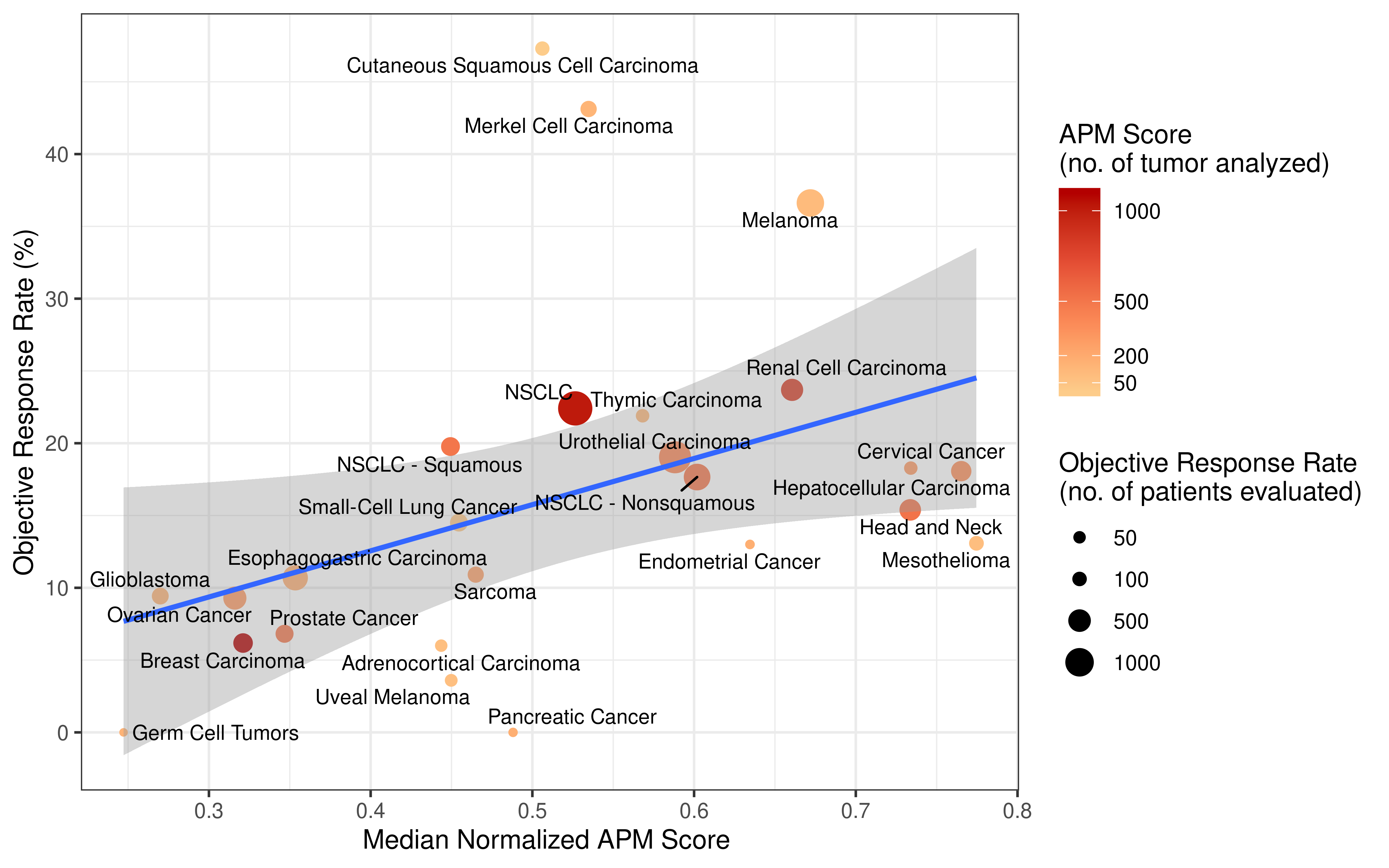
ggplot(sm_data, aes(x = Pool_TMB, y = Pool_ORR)) +
  geom_point(aes(color = Patients_TMB, size = Patients_ORR)) +
  geom_smooth(method = "lm", se = T) +
  geom_text_repel(aes(label = Cancer_Type), size = 3) +
  labs(
    x = "Median No. of Coding Somatic Mutation per MB", y = "Objective Response Rate (%)",
    size = "Objective Response Rate\n(no. of patients evaluated)",
    color = "Tumor Mutational Burden\n(no. of tumor analyzed)"
  ) +
  scale_x_continuous(
    trans = log_trans(),
    breaks = c(2, 10, 20, 30, 40, 50),
    labels = c(2, 10, 20, 30, 40, 50)
  ) +
  scale_size_continuous(breaks = c(50, 100, 500, 1000)) +
  scale_color_gradientn(
    colours = RColorBrewer::brewer.pal(5, name = "OrRd")[-1],
    breaks = c(100, 1000, 5000, 10000)
  ) +
  theme_bw() +
  guides(
    color = guide_colorbar(order = 1)
  )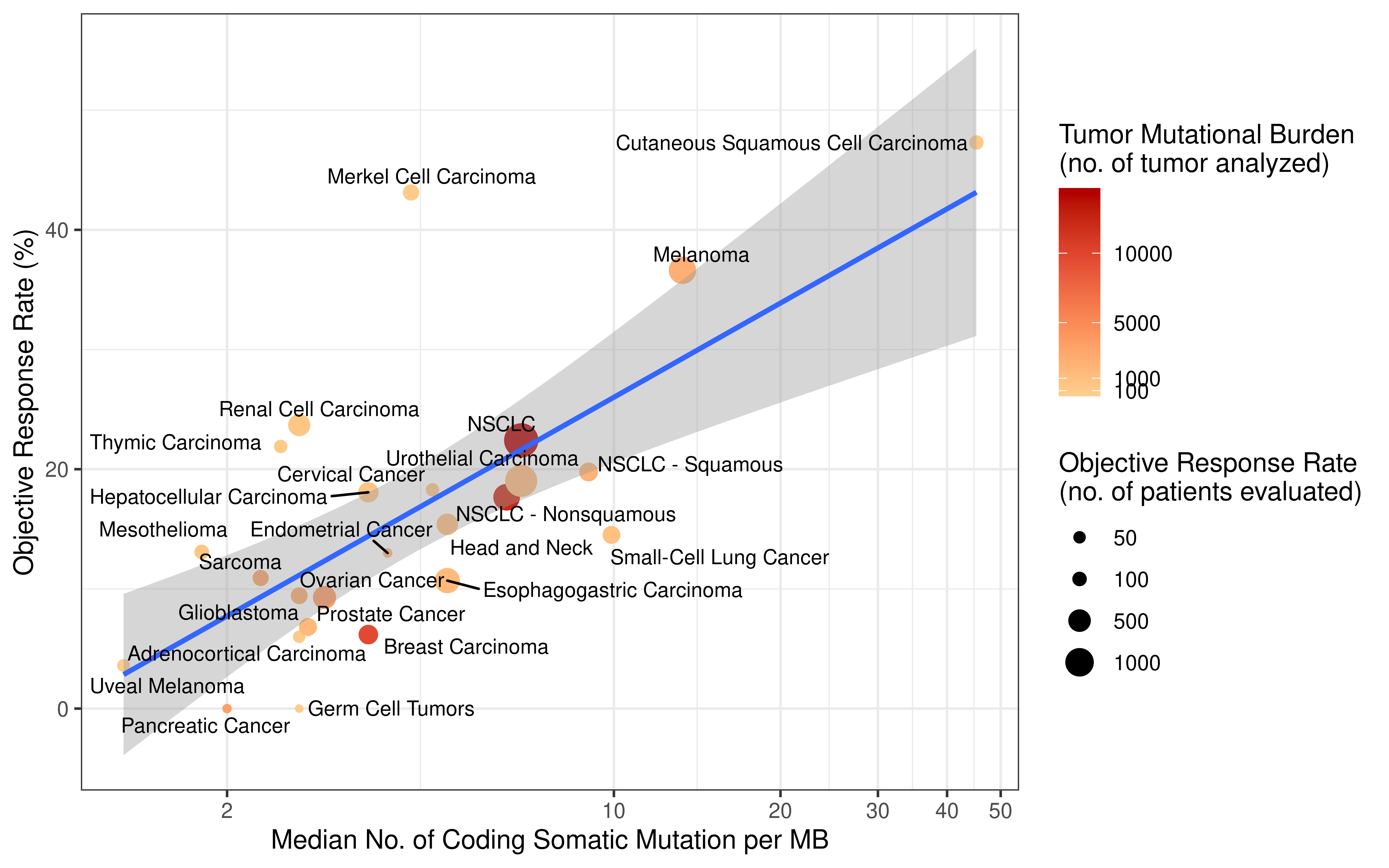
TIGS definition and performance
From the aspect of biological process, TMB release is independent from processing and presentation of tumor antigens. Now that we have found TMB and APM are biomarkers which can predict object reponse rate of cancer type in immunotherapy, these two factors are independent, and are both required for tumor immunogenicity determination, why not integrate them as a new biomarker which should be better than TMB?
Therefore, theoretically, tumor immunogenicity can be represented as
\[ [“Tumor \quad antigenicity”] \times [“Antigen \quad processing \quad and \quad presenting \quad status”]. \]
We use log(TMB) here because log(TMB) has been proved to have a linear relationship with ORR. So the formula can be written as
\[ TIGS = APS_{normalized} \times log(TMB) \]
However, some tumors have TMB level below 1 mutation/ Mb, to avoid minus number in quantifying “tumor antigenicity”, we add number 1 to all normalized TMB. So in this case, the TIGS formula is
\[ TIGS = APS_{normalized} \times log(TMB + 1) \]
When TMB < 1 mutation/Mb, the
log(TMB)would less than 0, if APS is very big, we would get a big minus number in this case, which against common sense.
Now we construct a linear model by integrate TMB and APM.
lm(Pool_ORR ~ log(Pool_TMB + 1):Pool_APM, data = sm_data) -> fit3

summary(fit3)
#>
#> Call:
#> lm(formula = Pool_ORR ~ log(Pool_TMB + 1):Pool_APM, data = sm_data)
#>
#> Residuals:
#>    Min     1Q Median     3Q    Max
#> -10.07  -4.26  -1.32   1.94  26.70
#>
#> Coefficients:
#>                            Estimate Std. Error t value Pr(>|t|)
#> (Intercept)                   -2.66       3.57   -0.75     0.46
#> log(Pool_TMB + 1):Pool_APM    21.39       3.64    5.88  5.4e-06 ***
#> ---
#> Signif. codes:  0 '***' 0.001 '**' 0.01 '*' 0.05 '.' 0.1 ' ' 1
#>
#> Residual standard error: 7.7 on 23 degrees of freedom
#> Multiple R-squared:  0.601,  Adjusted R-squared:  0.583
#> F-statistic: 34.6 on 1 and 23 DF,  p-value: 5.39e-06
We observe that 60.1% variance of ORR can be explained by TIGS, this result is indeed bettern than TMB.
sm_data$tigs <- sm_data$Pool_APM * log(sm_data$Pool_TMB + 1)

ggplot(sm_data, aes(x = tigs, y = Pool_ORR)) +
  geom_point(aes(size = Patients_ORR)) +
  geom_smooth(method = "lm", se = T) +
  geom_text_repel(aes(label = Cancer_Type), size = 3) +
  labs(
    x = "Tumor Immunogenicity Score ", y = "Objective Response Rate (%)",
    size = "Objective Response Rate\n(no. of patients evaluated)"
  ) +
  scale_size_continuous(breaks = c(50, 100, 500, 1000)) +
  theme_bw()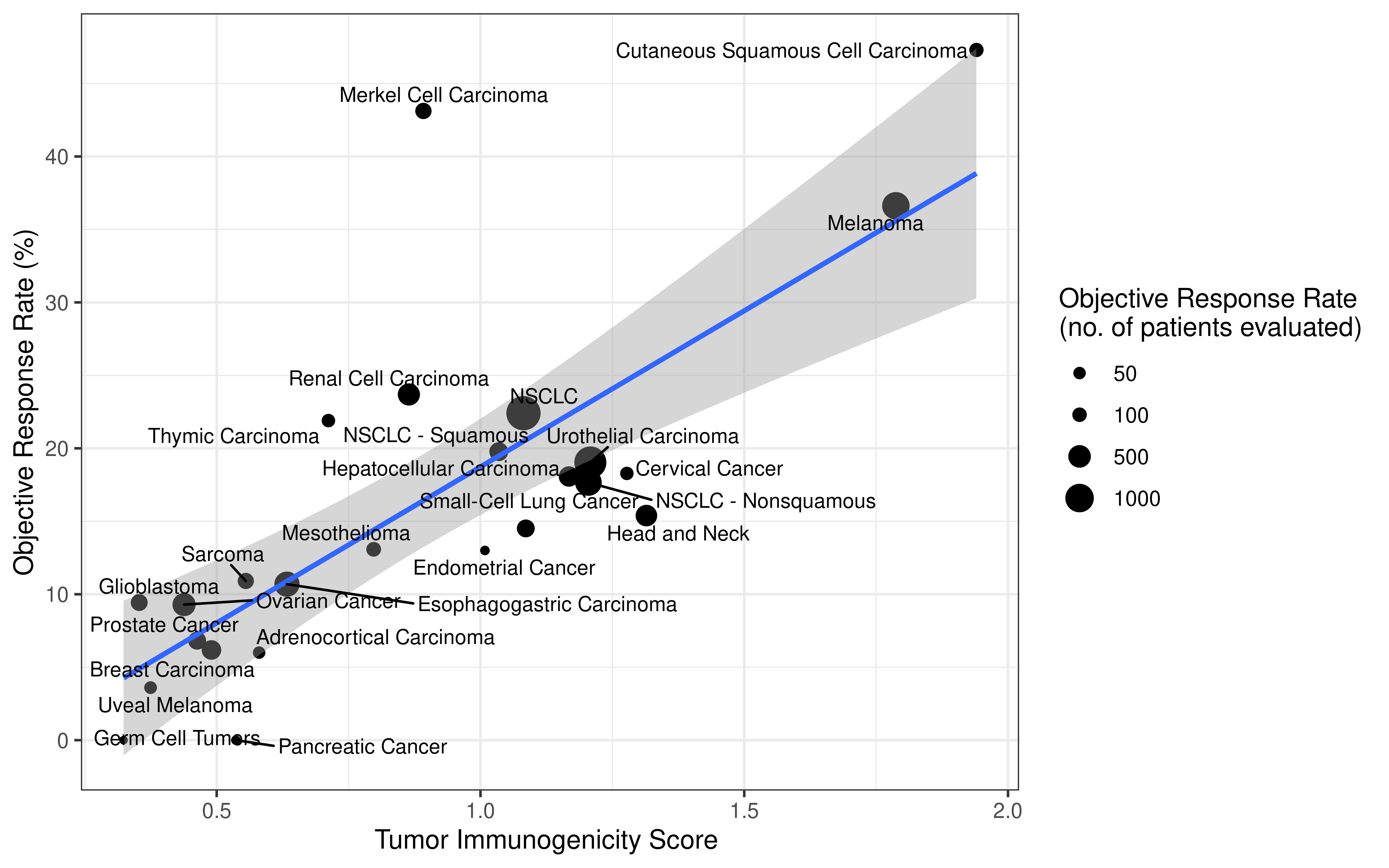
More exploration of TIGS formula
Would other combination of TMB and APS be better?
As mentioned above, we constructed the formula of TIGS according to our understanding of “tumor antigenicity”. Is there a better combination of these two factors?
There are two basic models we take into consideration.
- Model 1: \(ORR = a \times (APS \times log(TMB)) + b\), i.e. \(TIGS = APS \times log(TMB)\) (This is the model we used above)
- Model 2: \(ORR = e \times (a \times APS + b\times log(TMB) + c\times APS \times log(TMB)) + d\), i.e. \(TIGS = a \times APS + b\times log(TMB) + c\times APS \times log(TMB)\)
a, b, c, d and e here are coefficients. In R, we don’t need to write them in models, it will take care of them.
Now, let’s observe the results.
# Model 1
lm(Pool_ORR ~ log(Pool_TMB + 1):Pool_APM, data = sm_data) %>% summary()
#>
#> Call:
#> lm(formula = Pool_ORR ~ log(Pool_TMB + 1):Pool_APM, data = sm_data)
#>
#> Residuals:
#>    Min     1Q Median     3Q    Max
#> -10.07  -4.26  -1.32   1.94  26.70
#>
#> Coefficients:
#>                            Estimate Std. Error t value Pr(>|t|)
#> (Intercept)                   -2.66       3.57   -0.75     0.46
#> log(Pool_TMB + 1):Pool_APM    21.39       3.64    5.88  5.4e-06 ***
#> ---
#> Signif. codes:  0 '***' 0.001 '**' 0.01 '*' 0.05 '.' 0.1 ' ' 1
#>
#> Residual standard error: 7.7 on 23 degrees of freedom
#> Multiple R-squared:  0.601,  Adjusted R-squared:  0.583
#> F-statistic: 34.6 on 1 and 23 DF,  p-value: 5.39e-06
# Model 2
lm(Pool_ORR ~ log(Pool_TMB + 1) * Pool_APM, data = sm_data) %>% summary()
#>
#> Call:
#> lm(formula = Pool_ORR ~ log(Pool_TMB + 1) * Pool_APM, data = sm_data)
#>
#> Residuals:
#>    Min     1Q Median     3Q    Max
#>  -8.97  -4.22  -2.46   2.26  26.69
#>
#> Coefficients:
#>                            Estimate Std. Error t value Pr(>|t|)
#> (Intercept)                  -17.63      23.61   -0.75     0.46
#> log(Pool_TMB + 1)             12.17      15.51    0.78     0.44
#> Pool_APM                      24.04      45.06    0.53     0.60
#> log(Pool_TMB + 1):Pool_APM     1.02      29.21    0.03     0.97
#>
#> Residual standard error: 7.8 on 21 degrees of freedom
#> Multiple R-squared:  0.621,  Adjusted R-squared:  0.567
#> F-statistic: 11.5 on 3 and 21 DF,  p-value: 0.000114
Model 2 is a little better than model 1, however model 1 is much simpler (all terms of model 1 is included in model 2!). Following Occam’s razor, we choose model 1 when compare it with model 2.
Any promotion of formula \(TIGS = APS \times log(TMB + 1)\)?
We still have a question about TIGS formula. The TMB in formula is calculated as
\[ TMB = ln(\frac{whole \quad exome \quad mutation \quad number}{38} + 1 ) \]
We choose nonsynonymous mutations because they have functional effects. Only functional effects on protein will generate neo-antigen (peptide).
We use 38 here because 38 MB is the estimated length of exome, so we can normalize TMB to per MB. However, in math model, there may be a better value “a” than 38. We don’t know yet, so we need to explore this “a” value.
We simulate “a” value from 0.1 to 10000 with step size 0.1 in the following formula, the resulted TIGS is then used to fit a linear model for pan-cancer ICI ORR prediction. We calculate differnt R Square value under each “a” and see how it changes.
\[ TIGS = APS_{normalized} \times ln(\frac{whole \quad exome \quad mutation \quad number}{a} + 1) \]
Implementation:
df <- sm_data
df$APS <- df$Pool_APM
df$TMB <- df$Pool_TMB * 38 # transform back to whole exome nonsynonymous mutation number
df$ORR <- df$Pool_ORR

df <- dplyr::select(df, APS, TMB, ORR)


calcTrends <- function(df, a) {
  sapply(a, function(x, data) {
    summary(lm(ORR ~ APS:log((TMB / x + 1)), data = df))$r.squared
  }, data = df)
}Plot the simulation result.
opar <- par(no.readonly = TRUE)
par(mfrow = c(1, 2))
plot(res_df, las = 1, xlab = "a", ylab = "R Square", type = "l")
plot(res_df[1:1000, ], las = 1, xlab = "a", ylab = "R Square", type = "l")
abline(v = 38, lty = 2, col = "red")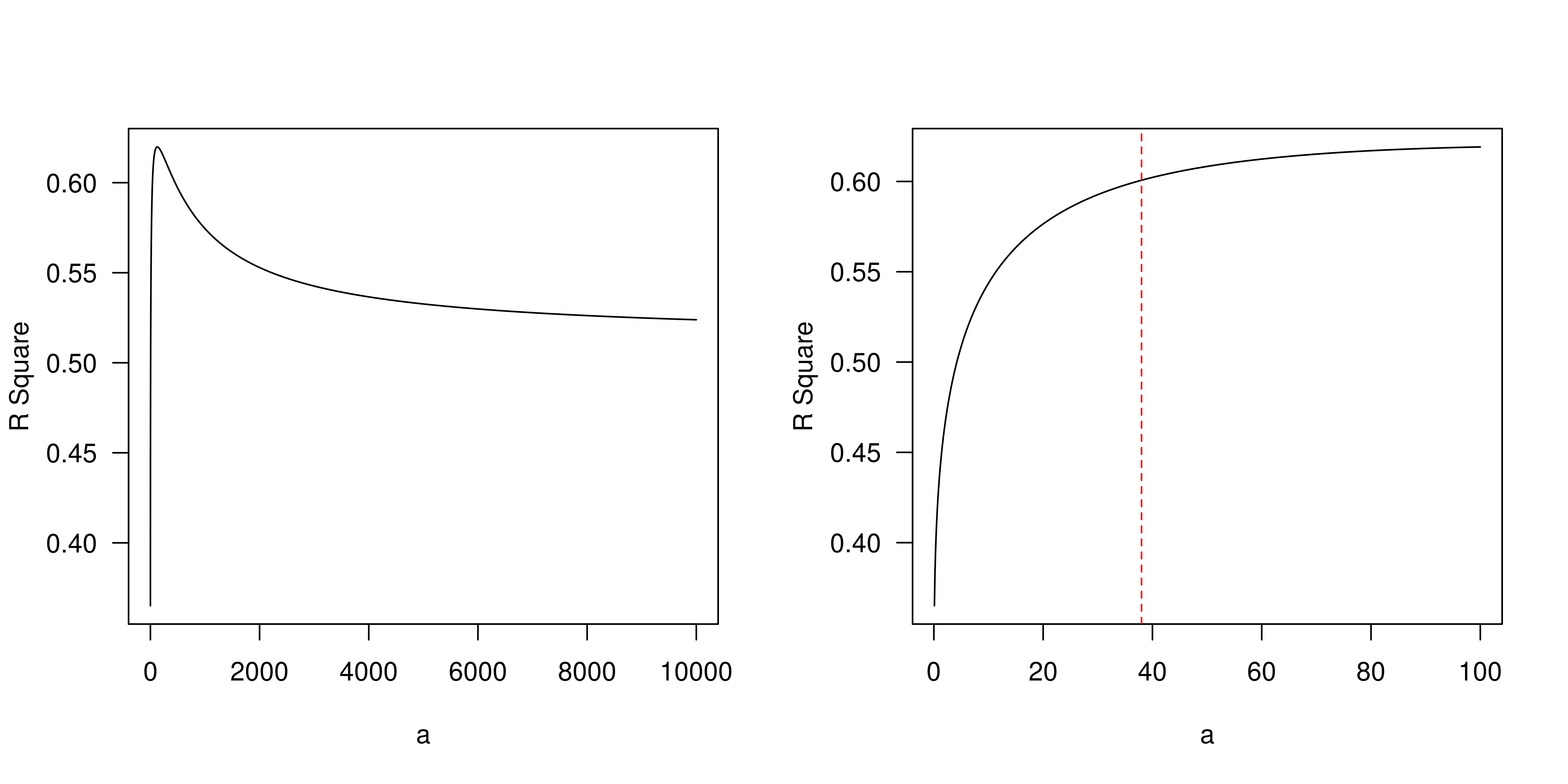
We can find that R squares of linear model have a maximum value when “a” is around 40. Therefore, “a=38” is optimized to rescale the raw whole exome mutation counts and balance the contribution for APM and TMB in TIGS formula.
Performance comparison on immunotherapy clinical response prediction and survival benefit
Description of datasets please see preprocessing part or “Method Section” of manuscript.
TMB is a well-known biomarker and has been applied. Considering our TIGS is based on TMB, thus the most important point we wanna do in this section is comparing the prediction/clinical perfermance between TMB and TIGS.
However, some other biomarkers can predict immunotherapy response have been studied by other groups. Therefore, this section we will include following biomarkers in comparsion.
- APS - antigen processing and presenting efficiency score
- TMB - tumor mutation burden
- TIGS - tumor immunogenicity score
- IIS - immune infiltration score
- IFNG - interferon gamma response biomarkers of 6 genes including IFNG, STAT1, IDO1, CXCL10, CXCL9, and HLA-DRA
- CD8 - gene expression level of CD8A + CD8B
- PDL1 - an immunohistochemistry (IHC) biomarker approved by FDA. This study we use PD-L1 gene expression as the IHC surrogate
- TIDE - TIDE signature which integrates the expression signatures of T cell dysfunction and T cell exclusion to model tumor immune evasion.
- ISG.RS and IFNG.GS signatures described in Benci et al, Cell 2019
- PHBR scores from MHC-I Genotype Restricts the Oncogenic Mutational Landscape and Evolutionary Pressure against MHC Class II Binding Cancer Mutations
The predicted values of gene expression biomarkers (i.e. IFNG, CD8, PDL1) are the average values among all members defined by the original publications. For ISG.RS and IFNG.GS, we follow the reference to calculate normlized score.
We will also try to combine these gene expression based signatures with TMB to see their performance.
Preprocessing of immunotherapy datasets
The first step is to preprocess 3 immunotherapy datasets with gene expression, TMB and clinical outcome available. APS from Pancan analysis is used to normalize APS here.
# get min and max APM value based on TCGA and GEO pan-cancer data
load("results/df_all.RData")
min_APS <- min(df_all$APM)
max_APS <- max(df_all$APM)
rm(df_all)

# load gene list
load("results/merged_geneList.RData")
# load function
source("../code/functions.R")
Hugo et al 2016 dataset
## Data source: Genomic and Transcriptomic Features of Response to Anti-PD-1 Therapy in Metastatic Melanoma. Cell 2016 Mar 24;165(1):35-44. PMID: 26997480
suppressPackageStartupMessages(library(GEOquery))
library(tidyverse)
library(readxl)
geo_dir <- "../data/GEOdata"

gse <- "GSE78220"
GSE_78220 <- getGEO(gse, GSEMatrix = TRUE, AnnotGPL = TRUE, destdir = geo_dir)
GSE_78220 <- GSE_78220$GSE78220_series_matrix.txt.gz

#### Download gene expression using following command
# download.file(url = "https://www.ncbi.nlm.nih.gov/geo/download/?acc=GSE78220&format=file&file=GSE78220%5FPatientFPKM%2Exlsx", destfile = "../data/GSE78220_FPKM.xlsx")

GSE78220_FPKM <- readxl::read_xlsx("../data/GSE78220_FPKM.xlsx")

GSE78220_FPKM <- GSE78220_FPKM %>%
  as.data.frame() %>%
  mutate(mean_expr = rowMeans(.[, -1], na.rm = TRUE)) %>%
  arrange(Gene, desc(mean_expr)) %>%
  distinct(Gene, .keep_all = TRUE) %>%
  dplyr::select(-mean_expr) %>%
  as.tibble()

# pData(GSE_78220) %>% View()

# normalize gene expression as log(x + 1)
GSE78220_Norm <- GSE78220_FPKM
GSE78220_Norm[, -1] <- log2(GSE78220_Norm[, -1] + 1)

# apply gsva
applyGSVA(merged_geneList,
  group_col = "Cell_type",
  gene_col = "Symbol", ExprMatList = list(GSE78220_Norm), method = "gsva"
) -> gsva.hugo2016

gsva.hugo2016 <- calc_TisIIs(gsva.hugo2016[[1]])

# normalize APS
APS_hugo <- gsva.hugo2016$APM
APS_hugo <- (APS_hugo - min_APS) / (max_APS - min_APS)

names(APS_hugo) <- colnames(GSE78220_Norm)[-1]
APS_hugo
names(APS_hugo) <- sub(pattern = "(Pt.*)\\.baseline", "\\1", names(APS_hugo))


# keep biggest value
APS_hugo <- APS_hugo[-21]
names(APS_hugo)[c(14, 20)] <- c("Pt16", "Pt27")
APS_hugo

# keep corresponding expression data for downstream analysis
rna_hugo <- GSE78220_Norm[, -22]
colnames(rna_hugo)[-1] <- names(APS_hugo)

if (!file.exists("results/Hugo2016_RNA.RData")) {
  save(rna_hugo, file = "results/Hugo2016_RNA.RData")
}

GSE78220.APS <- tibble(PatientID = names(APS_hugo), APS = APS_hugo, IIS = gsva.hugo2016$IIS[-21])

# generate results for random selected APS genes
set.seed(123456)
apm_gens <- merged_geneList %>% dplyr::filter(Cell_type == "APM")
sapply(1:100, function(i) {
  tempGens <- sample(GSE78220_Norm$Gene, 18)
  apm_gens$Symbol <- tempGens
  applyGSVA(apm_gens,
    group_col = "Cell_type",
    gene_col = "Symbol", ExprMatList = list(GSE78220_Norm), method = "gsva"
  )
}) -> gsva.hugo2016.random

gsva.hugo2016.random <- as.data.frame(sapply(gsva.hugo2016.random, function(x) {
  (x$APM - min_APS) / (max_APS - min_APS)
}))
colnames(gsva.hugo2016.random) <- paste0("APS", 1:100)
gsva.hugo2016.random <- gsva.hugo2016.random[-21, ]
rownames(gsva.hugo2016.random) <- names(APS_hugo)

# read clincal and tmb data
GSE_78220.TMB <- read_csv("../data/Cell2016.csv", col_types = cols())
GSE_78220.TMB$nTMB <- GSE_78220.TMB$TotalNonSyn / 38

info_hugo <- full_join(GSE_78220.TMB, GSE78220.APS, by = "PatientID")
info_hugo <- info_hugo[, c(1:5, 14:16, 13)]

# calculate TIGS score
info_hugo$TIGS <- log(info_hugo$nTMB) * info_hugo$APS

save(info_hugo, file = "results/Hugo2016_Info.RData")
Van Allen et al 2015 dataset
#----------------------------------------------------------
# Data source :
# Science 2015: Genomic correlates of response to CTLA4 blockade in metastatic melanoma
#--------------------------
library(readxl)
suppressPackageStartupMessages(library(tidyverse))
science2015_TMB <- read_xlsx("../data/Science2015_TMB_List_AllPatients.xlsx")
science2015_cli1 <- read_xlsx("../data/Science2015_Clinical.xlsx", sheet = 1)
science2015_cli2 <- read_xlsx("../data/Science2015_Clinical.xlsx", sheet = 2)
science2015_rna <- read_tsv("../data/MEL-IPI-Share.rpkm.gct", col_types = cols())

#---- Preprocess
vc.nonSilent <- c(
  "Frame_Shift_Del", "Frame_Shift_Ins", "Splice_Site", "Translation_Start_Site",
  "Nonsense_Mutation", "Nonstop_Mutation", "In_Frame_Del",
  "In_Frame_Ins", "Missense_Mutation"
)

science2015_TMB %>%
  group_by(patient) %>%
  summarise(
    TotalMutation = n(),
    TotalNonSyn = sum(Variant_Classification %in% vc.nonSilent),
    nTMB = TotalNonSyn / 38
  ) -> science2015_TMB_summary

#---- remove duplicate symbols of rna data
science2015_rna %>%
  mutate(symbol = sub("(.*)\\..*$", "\\1", Description)) %>%
  dplyr::select(-Name, -Description) %>%
  dplyr::select(symbol, everything()) %>%
  as.data.frame() %>%
  mutate(mean_expr = rowMeans(.[, -1], na.rm = TRUE)) %>%
  arrange(symbol, desc(mean_expr)) %>%
  distinct(symbol, .keep_all = TRUE) %>%
  dplyr::select(-mean_expr) %>%
  as.tibble() -> science2015_ge

length(intersect(science2015_ge$symbol, GSE78220_Norm$Gene))
# the gene number of science paper is bigger than hugo 2016
# maybe miRNA and some other RNA included
# keep them almost equal\
science2015_ge <- science2015_ge %>%
  filter(symbol %in% GSE78220_Norm$Gene)

science2015_ge[, -1] <- log2(science2015_ge[, -1] + 1)

applyGSVA(merged_geneList,
  group_col = "Cell_type",
  gene_col = "Symbol",
  ExprMatList = list(science2015_ge), method = "gsva"
) -> gsva.VanAllen2015

gsva.VanAllen2015 <- calc_TisIIs(gsva.VanAllen2015[[1]])

APS_VanAllen <- gsva.VanAllen2015$APM
names(APS_VanAllen) <- colnames(science2015_ge)[-1]
APS_VanAllen <- (APS_VanAllen - min_APS) / (max_APS - min_APS)

APS_VanAllen
names(APS_VanAllen) <- sub("^MEL.IPI_(.*)\\.Tumor.*$", "\\1", names(APS_VanAllen))
APS_VanAllen

rna_VanAllen <- science2015_ge
colnames(rna_VanAllen)[-1] <- names(APS_VanAllen)
## save gene experssion
if (!file.exists("results/VanAllen2015_RNA.RData")) {
  save(rna_VanAllen, file = "results/VanAllen2015_RNA.RData")
}

APS_VanAllen_df <- tibble(
  patient = names(APS_VanAllen), APS = APS_VanAllen,
  IIS = gsva.VanAllen2015$IIS
)


# generate results for random selected APS genes
set.seed(123456)
# apm_gens = merged_geneList %>% dplyr::filter(Cell_type == "APM")
sapply(1:100, function(i) {
  tempGens <- sample(science2015_ge$symbol, 18)
  apm_gens$Symbol <- tempGens
  applyGSVA(apm_gens,
    group_col = "Cell_type",
    gene_col = "Symbol", ExprMatList = list(science2015_ge), method = "gsva"
  )
}) -> gsva.VanAllen2015.random

gsva.VanAllen2015.random <- as.data.frame(sapply(gsva.VanAllen2015.random, function(x) {
  (x$APM - min_APS) / (max_APS - min_APS)
}))
colnames(gsva.VanAllen2015.random) <- paste0("APS", 1:100)
rownames(gsva.VanAllen2015.random) <- names(APS_VanAllen)


science2015_cli <- bind_rows(
  dplyr::select(
    science2015_cli1, patient, age_start, RECIST, overall_survival, progression_free, primary, group,
    histology, stage, gender, dead, progression, neos50
  ),
  dplyr::select(
    science2015_cli2, patient, age_start, RECIST, overall_survival, progression_free, primary,
    group, histology, stage, gender, dead, progression
  ) %>% filter(patient %in% c("Pat20", "Pat91"))
)
# combine three datasets
info_VanAllen <- full_join(full_join(science2015_cli, APS_VanAllen_df, by = "patient"),
  science2015_TMB_summary,
  by = "patient"
)

info_VanAllen$TIGS <- info_VanAllen$APS * log(info_VanAllen$nTMB + 1) # to avoid TIGS <0, TIGS = log(TMB +1) *APM for this dataset

save(info_VanAllen, file = "results/VanAllen2015_Info.RData")
Snyder et al 2017 dataset
#----------------------------------------------------------------
# Contribution of systemic and somatic factors to clinical response and resistance in urothelial cancer: an exploratory multi-omic analysis
#---------------------------------------------------------------
# Data Source: https://github.com/XSLiuLab/multi-omic-urothelial-anti-pdl1
# This is a fork repository, original link can also be found in this link

library(tidyverse)
uro_cli <- read_csv("../data/data_clinical.csv", col_types = cols())
uro_counts <- read_csv("../data/data_counts.csv", col_types = cols())
uro_variants <- read_csv("../data/data_variants.csv",
  col_types = "c??????"
)
uro_rna <- read_csv("../data/data_kallisto.csv", col_types = cols())
uro_rna_wide <- reshape2::dcast(uro_rna, gene_name ~ patient_id, value.var = "est_counts")

# try remove duplicated genes
uro_rna_wide %>%
  as.data.frame() %>%
  mutate(mean_expr = rowMeans(.[, -1], na.rm = TRUE)) %>%
  arrange(gene_name, desc(mean_expr)) %>%
  distinct(gene_name, .keep_all = TRUE) %>%
  dplyr::select(-mean_expr) %>%
  as.tibble() -> uro_rna_ge

length(intersect(uro_rna_ge$gene_name, GSE78220_FPKM$Gene))
uro_rna_ge <- dplyr::filter(uro_rna_ge, gene_name %in% GSE78220_FPKM$Gene)
uro_rna_ge_Norm <- uro_rna_ge
uro_rna_ge_Norm[, -1] <- log2(uro_rna_ge_Norm[, -1] + 1)

## apply GSVA
applyGSVA(merged_geneList,
  group_col = "Cell_type",
  gene_col = "Symbol", ExprMatList = list(uro_rna_ge_Norm), method = "gsva"
) -> gsva.Snyder

gsva.Snyder <- calc_TisIIs(gsva.Snyder[[1]])

APS_Snyder <- gsva.Snyder$APM
APS_Snyder <- (APS_Snyder - min_APS) / (max_APS - min_APS)

## save gene expression
rna_Snyder <- uro_rna_ge_Norm
if (!file.exists("results/Snyder2017_RNA.RData")) {
  save(rna_Snyder, file = "results/Snyder2017_RNA.RData")
}

APS_Snyder_df <- tibble(
  patient_id = colnames(uro_rna_ge_Norm)[-1],
  APS = APS_Snyder,
  IIS = gsva.Snyder$IIS
)

# generate results for random selected APS genes
set.seed(123456)
# apm_gens = merged_geneList %>% dplyr::filter(Cell_type == "APM")
sapply(1:100, function(i) {
  tempGens <- sample(uro_rna_ge_Norm$gene_name, 18)
  apm_gens$Symbol <- tempGens
  applyGSVA(apm_gens,
    group_col = "Cell_type",
    gene_col = "Symbol", ExprMatList = list(uro_rna_ge_Norm), method = "gsva"
  )
}) -> gsva.Snyder.random

gsva.Snyder.random <- as.data.frame(sapply(gsva.Snyder.random, function(x) {
  (x$APM - min_APS) / (max_APS - min_APS)
}))
colnames(gsva.Snyder.random) <- paste0("APS", 1:100)
rownames(gsva.Snyder.random) <- colnames(uro_rna_ge_Norm)[-1]

uro_cli_2 <- uro_cli %>%
  dplyr::select(patient_id, Age, Sex, is_benefit, is_benefit_os, os, `Alive Status`) %>%
  mutate(event = ifelse(`Alive Status` == "Y", 0, 1))

uro_tmb <- uro_variants %>%
  group_by(patient_id) %>%
  summarise(TMB = n(), Nonsyn = sum(!is.na(gene_name)), nTMB = TMB / 38) %>%
  mutate(patient_id = as.character(patient_id))

info_Snyder <- dplyr::full_join(uro_cli_2, dplyr::full_join(uro_tmb, APS_Snyder_df))
info_Snyder$TIGS <- info_Snyder$APS * log(info_Snyder$nTMB)

save(info_Snyder, file = "results/Snyder2017_Info.RData")


save(gsva.hugo2016.random, gsva.Snyder.random, gsva.VanAllen2015.random,
  file = "results/randomAPS.RData"
)
Prepare work for calculating other predictors
Load data firstly.
# library(tidyverse)
sigList <- read_csv("../data/ICBbiomarkerSignature.csv", comment = "#", col_types = cols())
load("results/Hugo2016_RNA.RData")
load("results/VanAllen2015_RNA.RData")
load("results/Snyder2017_RNA.RData")

ISG_IFNG <- read_csv("../data/ISG.RS_and_IFNG.GS.csv", comment = "#")
#> Parsed with column specification:
#> cols(
#>   Type = col_character(),
#>   GeneSymbol = col_character()
#> )
Add APS7
APS7.genes <- c(
  "B2M", "HLA-A", "HLA-B", "HLA-C",
  "TAP1", "TAP2", "TAPBP"
)

APS7 <- merged_geneList %>%
  dplyr::filter(Symbol %in% APS7.genes)

APS7.GSVA <- applyGSVA(APS7, group_col = "Cell_type", gene_col = "Symbol", ExprMatList = list(rna_hugo, rna_Snyder, rna_VanAllen), method = "gsva")

APS7.GSVA <- APS7.GSVA %>%
  setNames(c("Hugo2016", "Snyder2017", "VanAllen2015")) %>%
  purrr::map_df(function(x) {
    x %>%
      tibble::rownames_to_column() %>%
      dplyr::mutate(
        APM = scales::rescale(APM)
      )
  }, .id = "Study") %>%
  dplyr::rename(APS7 = APM)
Gene expression biomarkers for response to immune checkpoint blockade
This section we will describe how to calculate predicted value of gene signature biomarker using gene expression data.
Check if all gene signatures are in data.
all(sigList$Genes %in% rna_hugo$Gene)
#> [1] TRUE
all(sigList$Genes %in% rna_Snyder$gene_name)
#> [1] TRUE
all(sigList$Genes %in% rna_VanAllen$symbol)
#> [1] TRUE
all(ISG_IFNG$GeneSymbol %in% rna_hugo$Gene)
#> [1] FALSE
all(ISG_IFNG$GeneSymbol %in% rna_Snyder$gene_name)
#> [1] FALSE
all(ISG_IFNG$GeneSymbol %in% rna_VanAllen$symbol)
#> [1] FALSE
sigList <- ISG_IFNG %>%
rename(
Signature = Type,
Genes = GeneSymbol
) %>% # make consistent
dplyr::filter(Genes %in% purrr::reduce(list(rna_hugo$Gene, rna_Snyder$gene_name, rna_VanAllen$symbol), intersect)) %>% # 3 genes removed in this operation
dplyr::bind_rows(sigList)Next we retrieve all gene expression values and then calculate average.
rna_hugo_df <- rna_hugo %>%
  dplyr::filter(Gene %in% sigList$Genes)

rna_VanAllen_df <- rna_VanAllen %>%
  dplyr::filter(symbol %in% sigList$Genes) %>%
  rename(Gene = symbol)

rna_Snyder_df <- rna_Snyder %>%
  dplyr::filter(gene_name %in% sigList$Genes) %>%
  rename(Gene = gene_name)
Combine them with sigList, then transform these data.frame to long format, calculate mean gene expression and transform back to wide format.
rna_hugo_sigExpr <- rna_hugo_df %>%
  dplyr::right_join(sigList, by = c("Gene" = "Genes")) %>%
  tidyr::gather(key = "sample", value = "expression", -Gene, -Signature) %>%
  dplyr::group_by(sample, Signature) %>%
  dplyr::summarise(expression = mean(expression)) %>%
  tidyr::spread(key = Signature, value = expression) %>%
  dplyr::mutate(study = "Hugo2016") %>%
  dplyr::ungroup()

rna_VanAllen_sigExpr <- rna_VanAllen_df %>%
  dplyr::right_join(sigList, by = c("Gene" = "Genes")) %>%
  tidyr::gather(key = "sample", value = "expression", -Gene, -Signature) %>%
  dplyr::group_by(sample, Signature) %>%
  dplyr::summarise(expression = mean(expression)) %>%
  tidyr::spread(key = Signature, value = expression) %>%
  dplyr::mutate(study = "VanAllen2015") %>%
  dplyr::ungroup()

rna_Snyder_sigExpr <- rna_Snyder_df %>%
  dplyr::right_join(sigList, by = c("Gene" = "Genes")) %>%
  tidyr::gather(key = "sample", value = "expression", -Gene, -Signature) %>%
  dplyr::group_by(sample, Signature) %>%
  dplyr::summarise(expression = mean(expression)) %>%
  tidyr::spread(key = Signature, value = expression) %>%
  dplyr::mutate(study = "Snyder2017") %>%
  dplyr::ungroup()
Show results as tables.
DT::datatable(rna_hugo_sigExpr,
  options = list(scrollX = TRUE, keys = TRUE), rownames = FALSE,
  caption = "gene signature expression in Hugo 2016 dataset"
)
DT::datatable(rna_VanAllen_sigExpr,
  options = list(scrollX = TRUE, keys = TRUE), rownames = FALSE,
  caption = "gene signature expression in VanAllen 2015 dataset"
)
DT::datatable(rna_Snyder_sigExpr,
  options = list(scrollX = TRUE, keys = TRUE), rownames = FALSE,
  caption = "gene signature expression in Snyder 2017 dataset"
)
Lastly, merge the three result datasets for downstream analysis.
Input file generation for TIDE
TIDE is developed by Shirley Liu lab, software website is available at (http://tide.dfci.harvard.edu/). We can generate input file for TIDE and submit it to the website for TIDE score calculation.
Following suggestions provided at TIDE website, we firstly generate input files for three immunotherapy datasets .
rna_Snyder <- rna_Snyder %>%
  rename(Gene = gene_name)

rna_VanAllen <- rna_VanAllen %>%
  rename(Gene = symbol)

# normalized expression substract mean expression
generateInput <- function(df) {
  df %>%
    mutate(Ref = rowMeans(.[, -1])) %>%
    mutate_at(vars(-Gene, -Ref), `-`, quote(Ref)) %>% # f <- function(num, ref) num - !!ref
    select(-Ref) %>%
    column_to_rownames(var = "Gene") %>%
    as.data.frame()
}

TIDE_hugo <- generateInput(rna_hugo)
TIDE_VanAllen <- generateInput(rna_VanAllen)
TIDE_Snyder <- generateInput(rna_Snyder)


if (!file.exists("results/TIDE_input_hugo.tsv")) {
  write.table(TIDE_hugo, file = "results/TIDE_input_hugo.tsv", quote = FALSE, sep = "\t", row.names = TRUE, col.names = TRUE)
  write.table(TIDE_VanAllen, file = "results/TIDE_input_VanAllen.tsv", quote = FALSE, sep = "\t", row.names = TRUE, col.names = TRUE)
  write.table(TIDE_Snyder, file = "results/TIDE_input_Snyder.tsv", quote = FALSE, sep = "\t", row.names = TRUE, col.names = TRUE)
}

rm(list = ls())
Next we submit the three tsv file to TIDE website. Previous immunotherapy item is set as “No”. The result csv files are saved to report/results directory.
ROC comparison
This section we compare ROC (AUC value) of biomarkers for response prediction.
library(pROC)
#> Type 'citation("pROC")' for a citation.
#>
#> Attaching package: 'pROC'
#> The following objects are masked from 'package:stats':
#>
#>     cov, smooth, var
library(tidyverse)
# theme_set(theme_bw())
# library(cowplot)

#------------------------------------------
# Load data
load("results/Hugo2016_Info.RData")
load("results/VanAllen2015_Info.RData")
load("results/Snyder2017_Info.RData")
load("results/randomAPS.RData")

load("results/GEBiomarker.RData")
load("results/APS_alternative.GSVA.RData")

# Of note, output csv from TIDE website has extra "" in last line
#          please remove it before load data
TIDE_hugo <- read_csv("results/TIDE_output_hugo.csv", col_types = cols())
TIDE_Snyder <- read_csv("results/TIDE_output_Snyder.csv", col_types = cols())
TIDE_VanAllen <- read_csv("results/TIDE_output_VanAllen.csv", col_types = cols())

#------------------------------------------
# Hugo 2016
info_hugo <- info_hugo %>%
  dplyr::left_join(dplyr::filter(GEBiomarker, study == "Hugo2016") %>%
                     dplyr::select(-study), by = c("PatientID" = "sample")) %>%
  dplyr::left_join(TIDE_hugo %>% dplyr::select(Patient, TIDE), by = c("PatientID" = "Patient")) %>%  # Combine APS7
  dplyr::left_join(APS7.GSVA %>%
                     dplyr::select(rowname, APS7),
                   by = c("PatientID" = "rowname")) %>%
  dplyr::rename(APS7_Sig = APS7) %>%  # differ from APS random
  dplyr::left_join(APS_MHC_II.GSVA %>%
                     dplyr::select(rowname, APS_MHC_II),
                   by = c("PatientID" = "rowname"))


# combine random data
gsva.hugo2016.random %>%
  rownames_to_column(var = "PatientID") %>%
  full_join(info_hugo, by = "PatientID") -> info_hugo

# Because less TIDE shows better outcome and
# Ref says ISG resistance signature (ISG.RS) is also associated with resistance to ICB
# We need reverse their score
# scale them to [0, 1]
# Then combine TMB with gene expression based markers
info_hugo = info_hugo %>%
  dplyr::mutate(
    TIDE = -TIDE,
    ISG.RS = -ISG.RS
  ) %>%
  dplyr::mutate_at(c("CD8", "IFNG", "IFNG.GS", "ISG.RS",
                     "PDL1", "TIDE", "APS7_Sig", "APS_MHC_II"), scales::rescale) %>%
  dplyr::mutate_at(c("CD8", "IFNG", "IFNG.GS", "ISG.RS",
                     "PDL1", "TIDE", "APS7_Sig", "APS_MHC_II"),
                   list(comb_TMB= ~ . * log(nTMB+1)))

genROC = function(info, markers, response="Response", direction="<", APSrandom=1:100) {
  ROC_LIST = list()
  # Calc APS random
  APSrandom_list = paste0("APS", APSrandom)
  for (i in c(markers,APSrandom_list)) {
    message(i)
    ROC_LIST[[i]] = roc(info[[response]], info[[i]], direction="<")
  }
  ROC_LIST
}

suppressMessages(
  hugo2016_roc <- genROC(info_hugo, markers = setdiff(colnames(info_hugo)[106:126],
                                                   "Treatment"))
)

#---------------------------
# VanAllen 2015

info_VanAllen <- info_VanAllen %>%
  dplyr::left_join(dplyr::filter(GEBiomarker, study == "VanAllen2015") %>%
                     dplyr::select(-study), by = c("patient" = "sample")) %>%
  dplyr::left_join(TIDE_VanAllen %>% dplyr::select(Patient, TIDE), by = c("patient" = "Patient")) %>%
  dplyr::left_join(APS7.GSVA %>%
                     dplyr::select(rowname, APS7),
                   by = c("patient" = "rowname")) %>%
  dplyr::rename(APS7_Sig = APS7) %>%  # differ from APS random
  dplyr::left_join(APS_MHC_II.GSVA %>%
                     dplyr::select(rowname, APS_MHC_II),
                   by = c("patient" = "rowname"))

info_VanAllen2 <- info_VanAllen %>%
  mutate(Response = case_when(
    group == "response" ~ "R",
    group == "nonresponse" ~ "NR",
    TRUE ~ NA_character_
  )) %>%
  filter(!is.na(Response))


## -- using following command if only compare patients with TIGS availble
## -- the result are basically same
# info_VanAllen2 = info_VanAllen %>%
#     mutate(Response = case_when(
#         group == "response" ~ "R",
#         group == "nonresponse" ~"NR",
#         TRUE ~ NA_character_
#     )) %>% filter(!is.na(Response), !is.na(TIGS))

# combine random data
gsva.VanAllen2015.random %>%
  rownames_to_column(var = "patient") %>%
  full_join(info_VanAllen2, by = "patient") -> info_VanAllen2

info_VanAllen2 = info_VanAllen2 %>%
  dplyr::mutate(
    TIDE = -TIDE,
    ISG.RS = -ISG.RS
  ) %>%
  dplyr::mutate_at(c("CD8", "IFNG", "IFNG.GS", "ISG.RS",
                     "PDL1", "TIDE", "APS7_Sig", "APS_MHC_II"), scales::rescale) %>%
  dplyr::mutate_at(c("CD8", "IFNG", "IFNG.GS", "ISG.RS",
                     "PDL1", "TIDE", "APS7_Sig", "APS_MHC_II"),
                   list(comb_TMB= ~ . * log(nTMB+1)))


suppressMessages(
  van2015_roc <- genROC(info_VanAllen2,
                     markers = setdiff(colnames(info_VanAllen2)[114:136],
                                       c("TotalMutation", "TotalNonSyn", "Response")))
)

#---------------------------------------
# Snyder 2017

info_Snyder <- info_Snyder %>%
  dplyr::left_join(dplyr::filter(GEBiomarker, study == "Snyder2017") %>%
                     dplyr::select(-study), by = c("patient_id" = "sample")) %>%
  dplyr::left_join(TIDE_Snyder %>% dplyr::select(Patient, TIDE), by = c("patient_id" = "Patient")) %>%
  dplyr::left_join(APS7.GSVA %>%
                     dplyr::select(rowname, APS7),
                   by = c("patient_id" = "rowname")) %>%
  dplyr::rename(APS7_Sig = APS7) %>%  # differ from APS random
  dplyr::left_join(APS_MHC_II.GSVA %>%
                     dplyr::select(rowname, APS_MHC_II),
                   by = c("patient_id" = "rowname"))

# combine random data
gsva.Snyder.random %>%
  rownames_to_column(var = "patient_id") %>%
  full_join(info_Snyder, by = "patient_id") -> info_Snyder

info_Snyder = info_Snyder %>%
  dplyr::mutate(
    TIDE = -TIDE,
    ISG.RS = -ISG.RS
  ) %>%
  dplyr::mutate_at(c("CD8", "IFNG", "IFNG.GS", "ISG.RS",
                     "PDL1", "TIDE", "APS7_Sig", "APS_MHC_II"), scales::rescale) %>%
  dplyr::mutate_at(c("CD8", "IFNG", "IFNG.GS", "ISG.RS",
                     "PDL1", "TIDE", "APS7_Sig", "APS_MHC_II"),
                   list(comb_TMB= ~ . * log(nTMB+1)))

suppressMessages(
  snyder2017_roc <- genROC(info_Snyder,
                     markers = colnames(info_Snyder)[111:130], response = "is_benefit")
)


ggroc(list(TMB = van2015_roc$nTMB, TIGS = van2015_roc$TIGS, TIDE = van2015_roc$TIDE),
  legacy.axes = TRUE
) +
  labs(color = "Predictor") +
  ggpubr::theme_classic2(base_size = 12)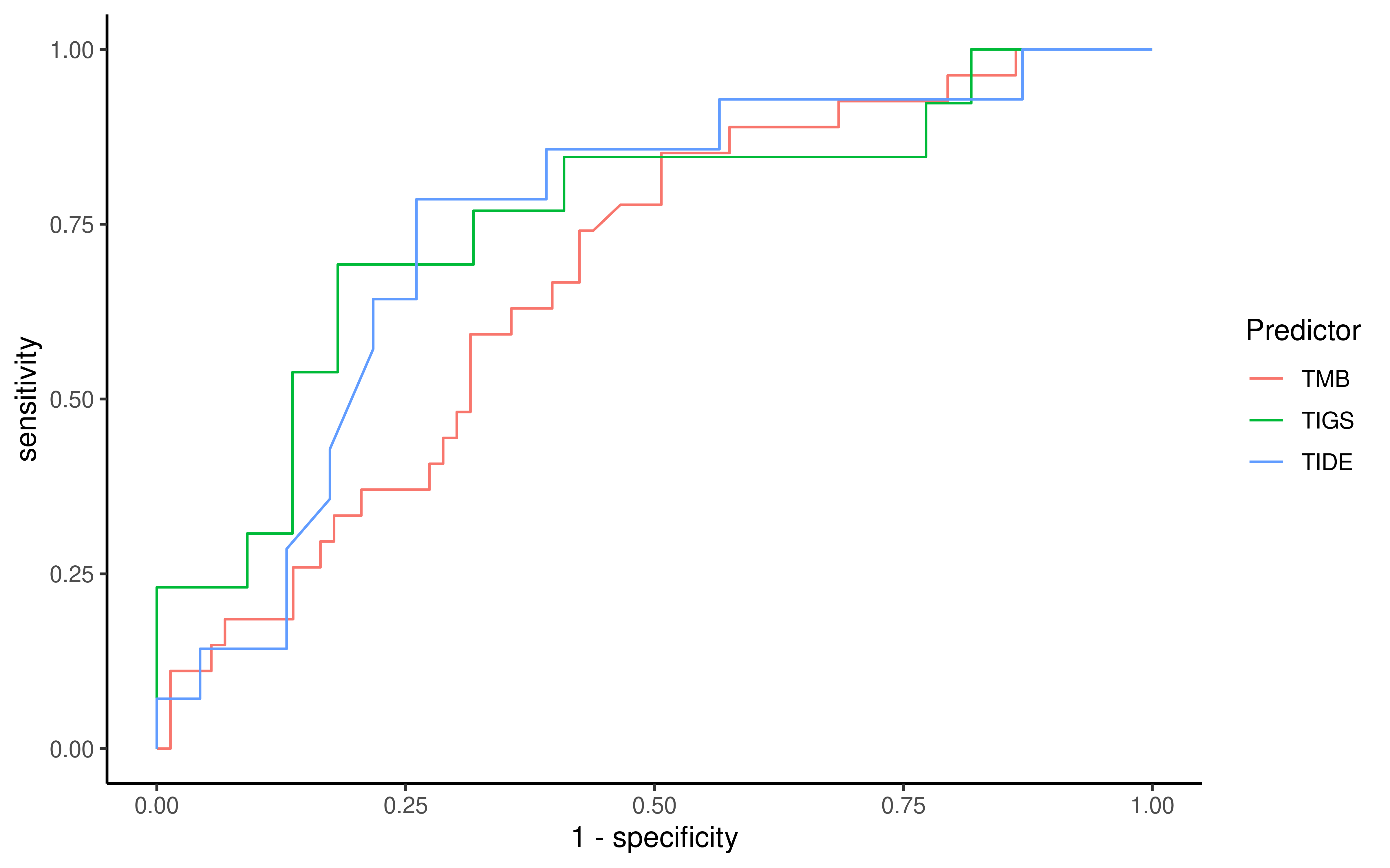
ggroc(list(TMB = hugo2016_roc$nTMB, TIGS = hugo2016_roc$TIGS, TIDE = hugo2016_roc$TIDE),
  legacy.axes = TRUE
) +
  labs(color = "Predictor") +
  ggpubr::theme_classic2(base_size = 12)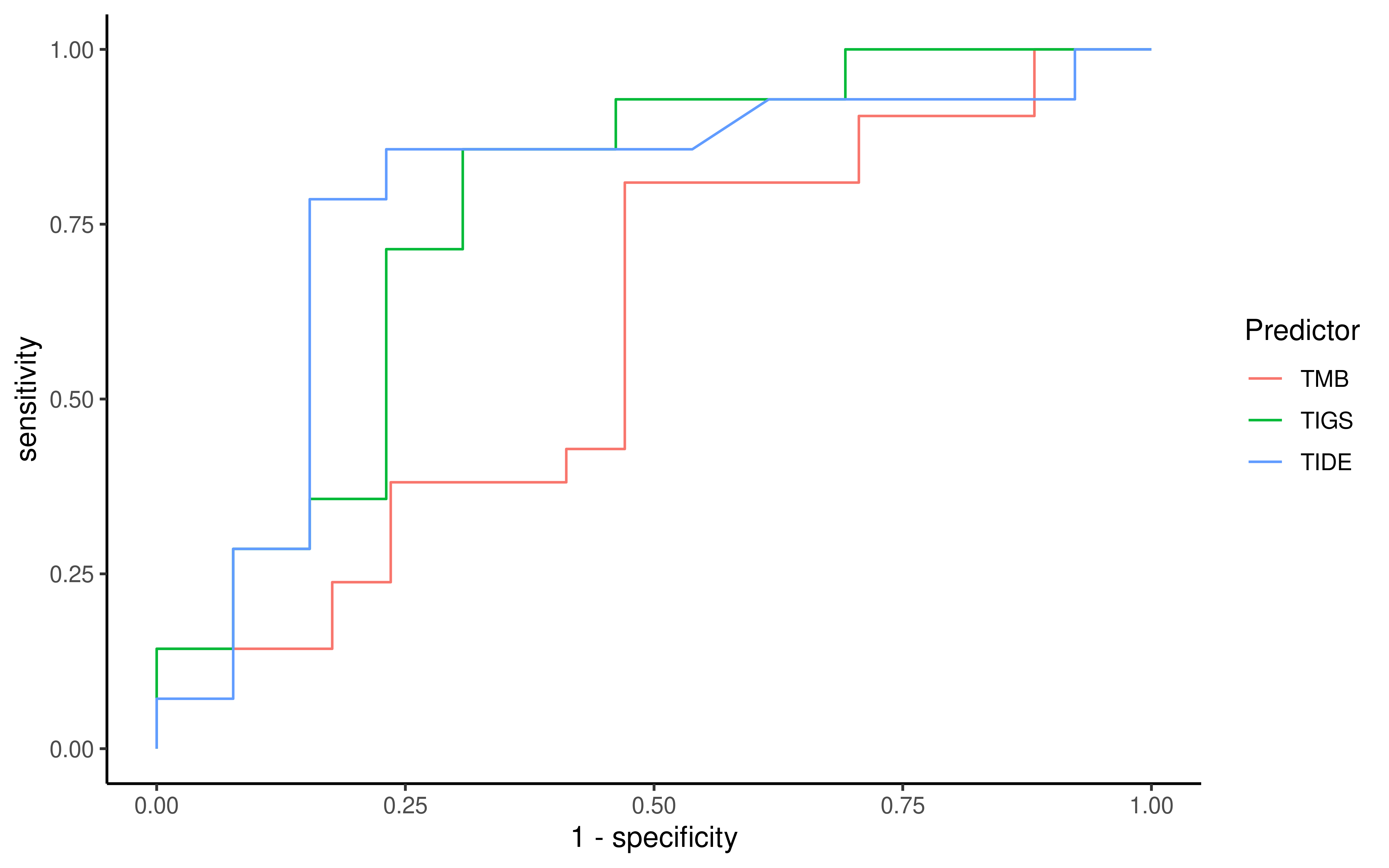
ggroc(list(TMB = snyder2017_roc$nTMB, TIGS = snyder2017_roc$TIGS, TIDE = snyder2017_roc$TIDE),
  legacy.axes = TRUE
) +
  labs(color = "Predictor") +
  ggpubr::theme_classic2(base_size = 12)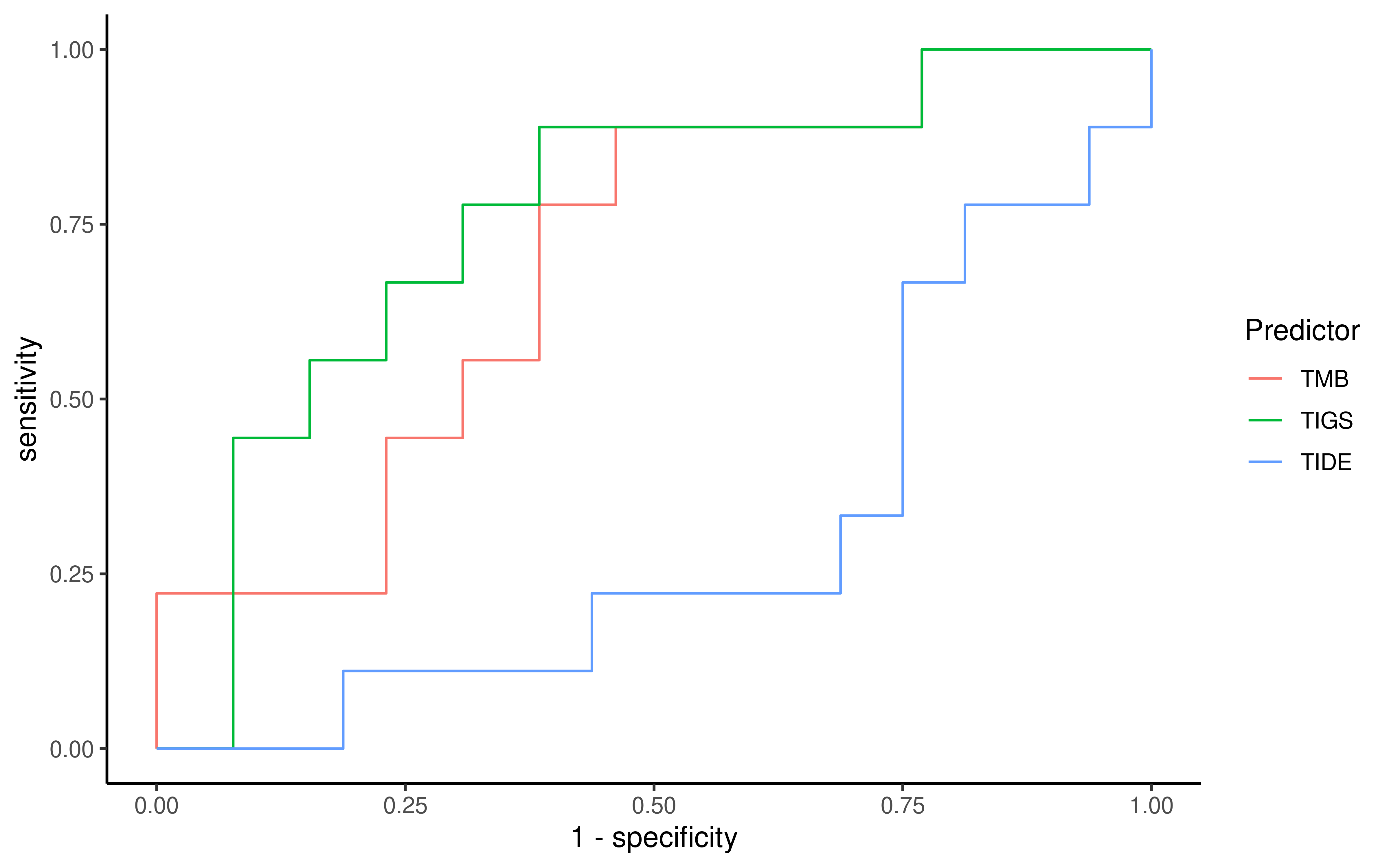
save(info_VanAllen2, info_hugo, info_Snyder, file = "results/data_for_ICB_ROC.RData")
save(van2015_roc, hugo2016_roc, snyder2017_roc, file = "results/ROC_ObjList.RData")
From comparison of AUC value above, we can conclude that:
- TIGS and TIDE are better than TMB
- TIGS and TIDE have almost same performance in two melanoma datasets, however, performance of TIDE go down a little in urothelial cancer dataset, maybe resulting from the fact that TIDE is trained on data of melanoma and NSCLC cancer (this point is stated at TIDE website, cancer type except for melanoma and NSCLC may not work).
- APS, TMB are also not bad predictors (they have almost same performance)
- Other predictors are not good predictors, they perform differently in different datasets.
Next, we summary results above for final visualization.
# summary AUC
van2015_auc = lapply(van2015_roc, function(x) as.numeric(auc(x)))
hugo2016_auc = lapply(hugo2016_roc, function(x) as.numeric(auc(x)))
snyder2017_auc = lapply(snyder2017_roc, function(x) as.numeric(auc(x)))
auc_df = list(van2015_auc, hugo2016_auc, snyder2017_auc) %>%
  dplyr::bind_rows() %>%
  dplyr::mutate(Group = c("VanAllen2015", "Hugo2016", "Snyder2017"),
                APSr = rowMeans(select(., paste0("APS", 1:100)))) %>%
  dplyr::rename(TMB = nTMB)

# Show AUC table
DT::datatable(auc_df,
  options = list(scrollX = TRUE, keys = TRUE), rownames = FALSE,
  caption = "AUC of biomarkers for response prediction in three ICB datasets"
)
Survival comparison
Above we already show APS, TMB, TIGS and TIDE are good predictors, this section we focus on them. We use cox model and separate patients into High and Low group in K-M survival analysis based on median biomarker predicted value.
library(survival)
library(survminer)

#----------------------
# Hugo 2016
hugo_os <- read_csv("../data/cell2016_OS.csv", col_types = cols())
info_hugo <- full_join(info_hugo, hugo_os, by = "PatientID")

# Cox model

# Cox result of TMB
coxph(Surv(OverallSurvival, VitalStatus == "Dead") ~ nTMB, data = info_hugo)
#> Call:
#> coxph(formula = Surv(OverallSurvival, VitalStatus == "Dead") ~
#>     nTMB, data = info_hugo)
#>
#>       coef exp(coef) se(coef)  z   p
#> nTMB -0.03      0.97     0.02 -1 0.2
#>
#> Likelihood ratio test=3  on 1 df, p=0.08
#> n= 37, number of events= 19
#>    (1 observation deleted due to missingness)

# Cox result of APS
coxph(Surv(OverallSurvival, VitalStatus == "Dead") ~ APS, data = info_hugo)
#> Call:
#> coxph(formula = Surv(OverallSurvival, VitalStatus == "Dead") ~
#>     APS, data = info_hugo)
#>
#>     coef exp(coef) se(coef)  z   p
#> APS -2.0       0.1      1.5 -1 0.2
#>
#> Likelihood ratio test=2  on 1 df, p=0.2
#> n= 26, number of events= 12
#>    (12 observations deleted due to missingness)

# Cox result of TIGS
coxph(Surv(OverallSurvival, VitalStatus == "Dead") ~ TIGS, data = info_hugo)
#> Call:
#> coxph(formula = Surv(OverallSurvival, VitalStatus == "Dead") ~
#>     TIGS, data = info_hugo)
#>
#>      coef exp(coef) se(coef)  z    p
#> TIGS -1.2       0.3      0.6 -2 0.03
#>
#> Likelihood ratio test=6  on 1 df, p=0.02
#> n= 26, number of events= 12
#>    (12 observations deleted due to missingness)

# Cox result of TIDE
coxph(Surv(OverallSurvival, VitalStatus == "Dead") ~ TIDE, data = info_hugo)
#> Call:
#> coxph(formula = Surv(OverallSurvival, VitalStatus == "Dead") ~
#>     TIDE, data = info_hugo)
#>
#>      coef exp(coef) se(coef)    z   p
#> TIDE -0.7       0.5      1.3 -0.5 0.6
#>
#> Likelihood ratio test=0.3  on 1 df, p=0.6
#> n= 26, number of events= 12
#>    (12 observations deleted due to missingness)


# K-M fit
info_hugo %>% # take care of NA values
  mutate(
    APS_Status = ifelse(APS > median(APS, na.rm = TRUE), "High",
      ifelse(is.na(APS), NA, "Low")
    ),
    # We reverse TIDE (do TIDE=-TIDE) in previous step
    # so here, we need to change the order
    TIDE_Status = ifelse(TIDE < median(TIDE, na.rm = TRUE), "High",
      ifelse(is.na(TIDE), NA, "Low")
    ),
    TMB_Status = ifelse(nTMB > median(nTMB), "High", "Low"),
    TIGS_Status = ifelse(TIGS > median(TIGS, na.rm = TRUE), "High",
      ifelse(is.na(TIGS), NA, "Low")
    )
  ) -> info_hugo2

# effect of TMB status on survival
fit1 <- survfit(Surv(OverallSurvival, VitalStatus == "Dead") ~ TMB_Status, data = info_hugo2)
ggsurvplot(fit1,
  data = info_hugo2, pval = TRUE, fun = "pct",
  xlab = "Time (in days)"
)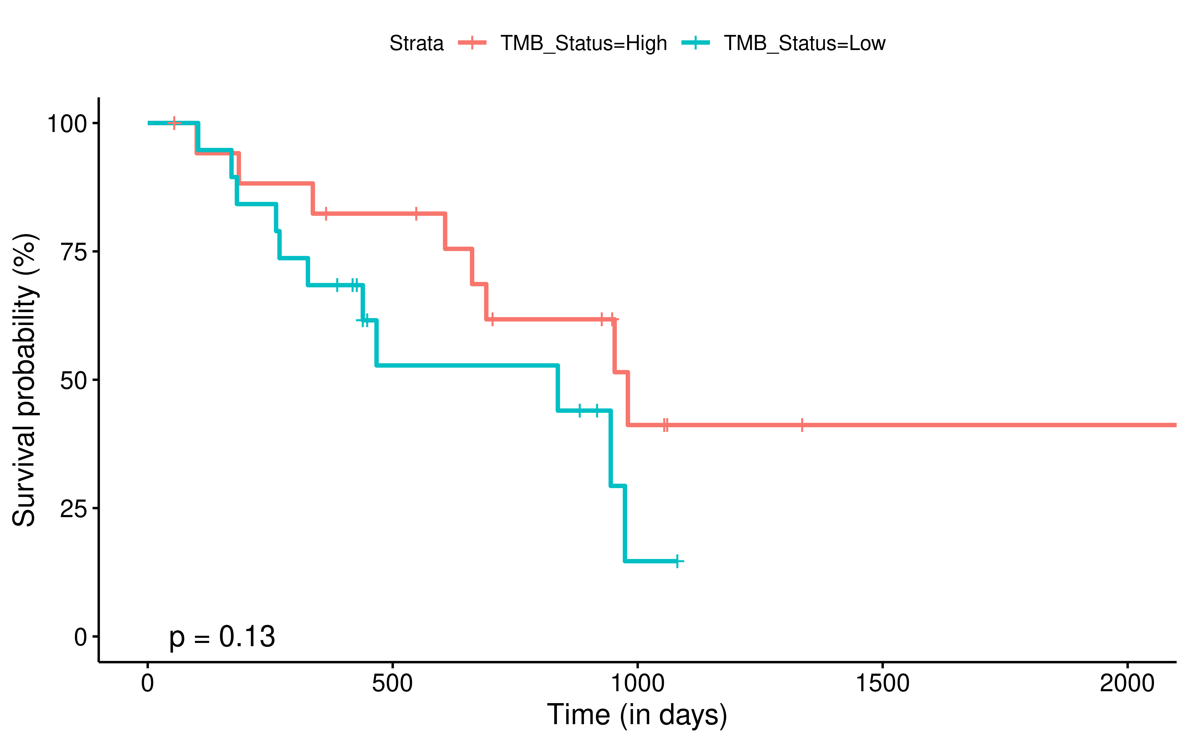
# effect of TIGS status on survival
fit2 <- survfit(Surv(OverallSurvival, VitalStatus == "Dead") ~ TIGS_Status, data = info_hugo2)
ggsurvplot(fit2, data = info_hugo2, pval = TRUE, fun = "pct", xlab = "Time (in days)")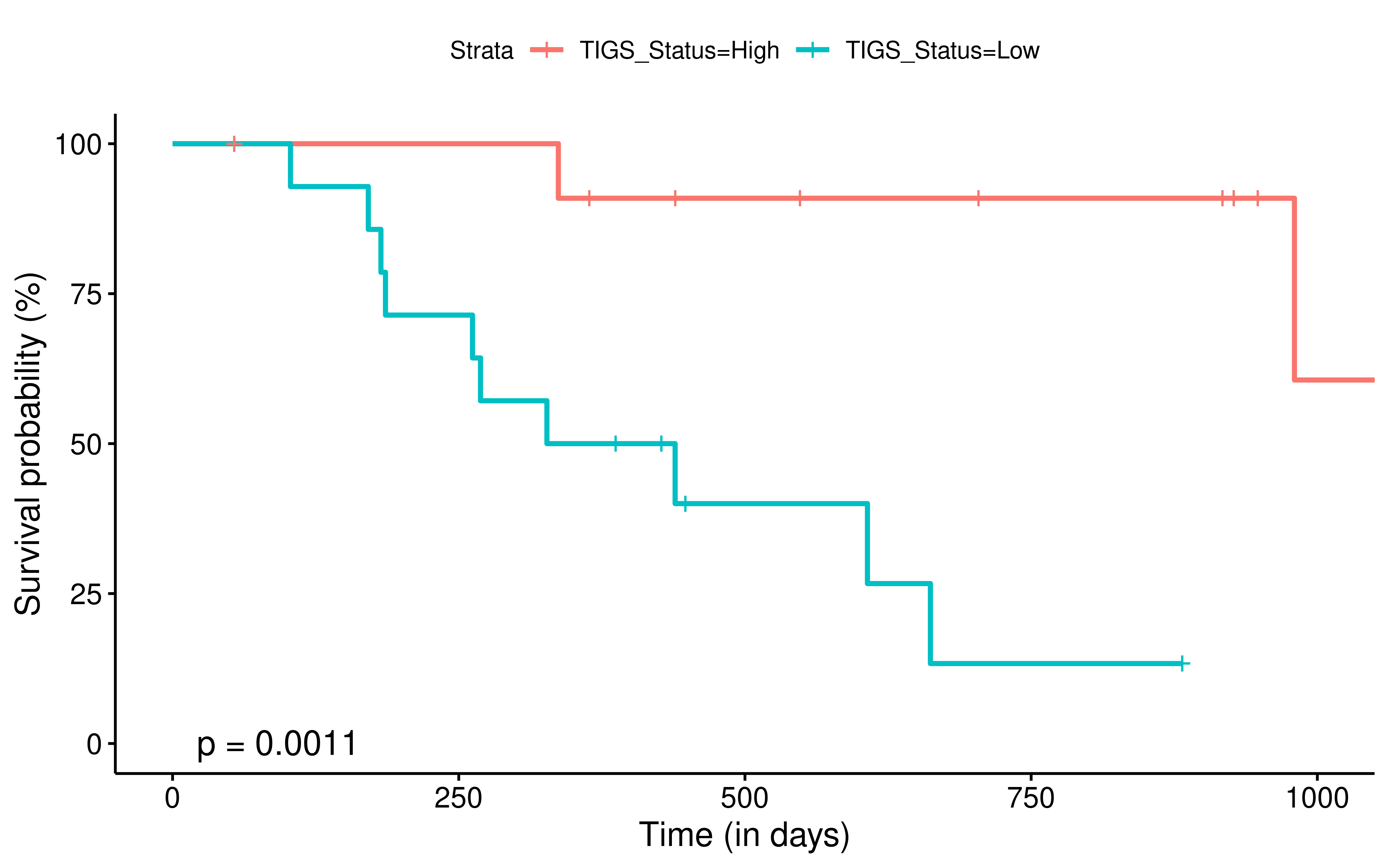
# effect of APS status on survival
fit3 <- survfit(Surv(OverallSurvival, VitalStatus == "Dead") ~ APS_Status, data = info_hugo2)
ggsurvplot(fit3,
  data = info_hugo2, pval = TRUE, fun = "pct",
  xlab = "Time (in days)"
)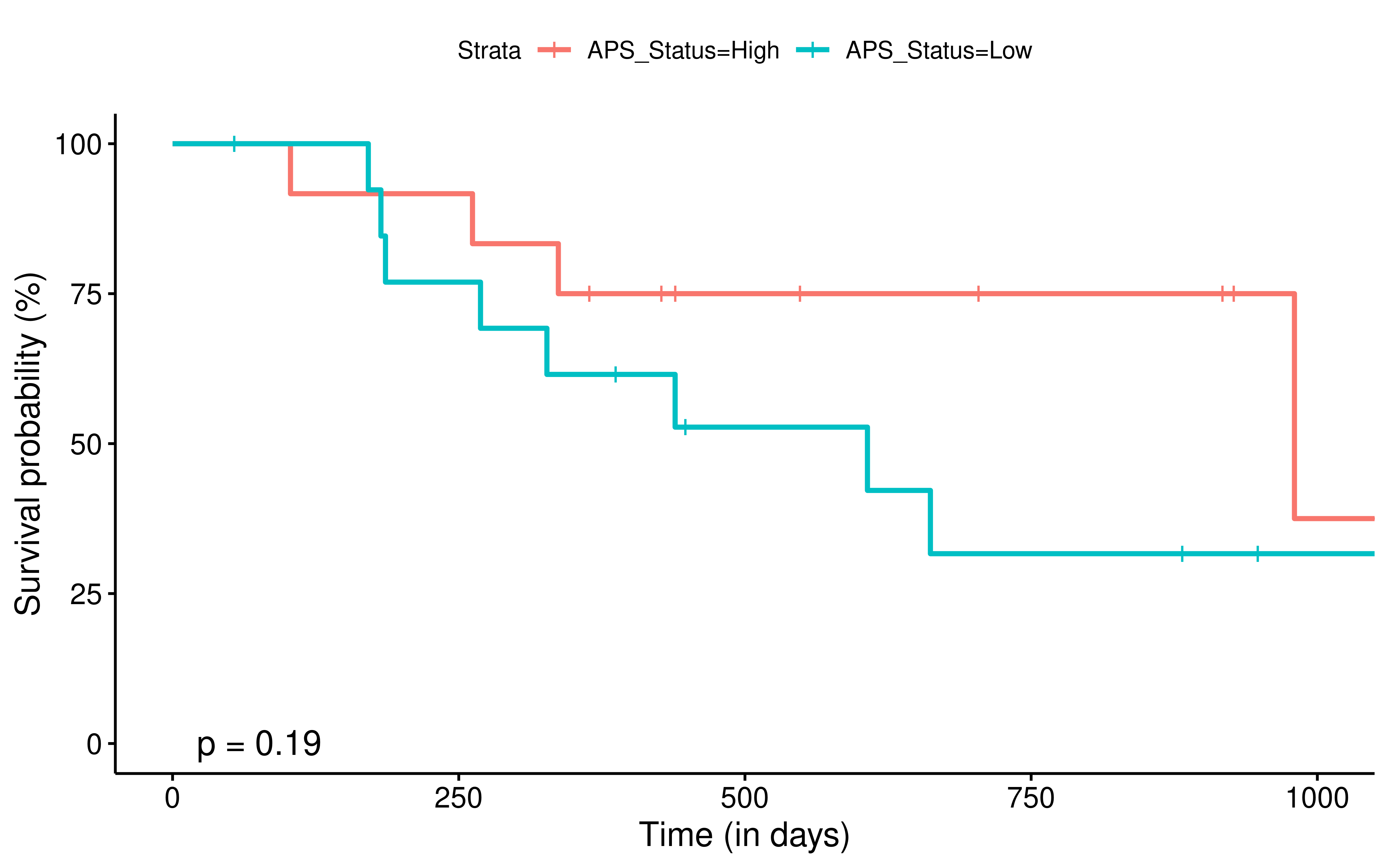
# effect of TIDE status on survival
fit4 <- survfit(Surv(OverallSurvival, VitalStatus == "Dead") ~ TIDE_Status, data = info_hugo2)
ggsurvplot(fit4, data = info_hugo2, pval = TRUE, fun = "pct", xlab = "Time (in days)")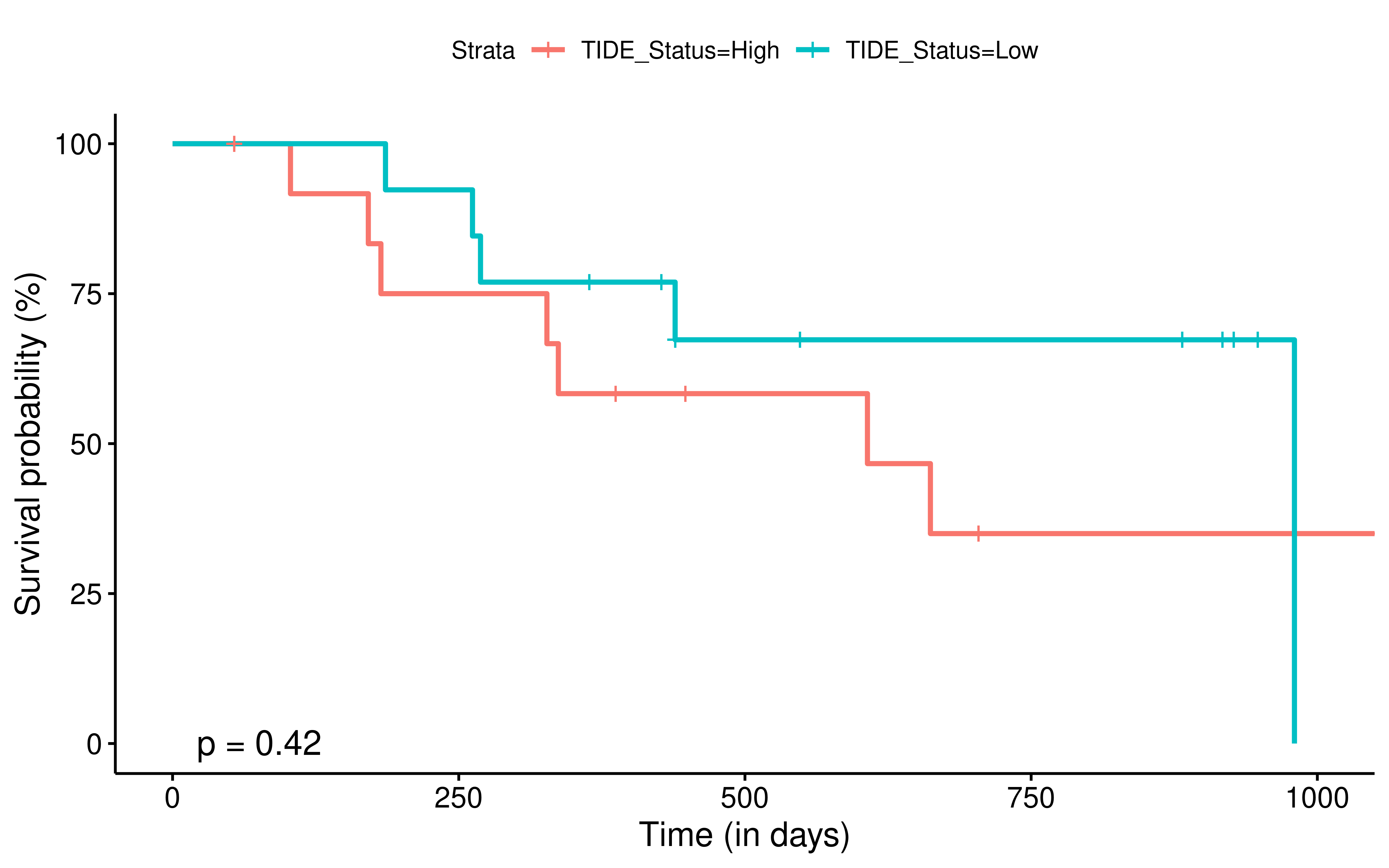
#----------------------
# Van Allen 2015

# Cox model

# Cox result of TMB
coxph(Surv(overall_survival, dead == 1) ~ nTMB, data = info_VanAllen)
#> Call:
#> coxph(formula = Surv(overall_survival, dead == 1) ~ nTMB, data = info_VanAllen)
#>
#>        coef exp(coef) se(coef)  z   p
#> nTMB -0.007     0.993    0.006 -1 0.2
#>
#> Likelihood ratio test=2  on 1 df, p=0.2
#> n= 110, number of events= 83
#>    (2 observations deleted due to missingness)

# Cox result of APS
coxph(Surv(overall_survival, dead == 1) ~ APS, data = info_VanAllen)
#> Call:
#> coxph(formula = Surv(overall_survival, dead == 1) ~ APS, data = info_VanAllen)
#>
#>     coef exp(coef) se(coef)  z    p
#> APS -1.7       0.2      0.8 -2 0.03
#>
#> Likelihood ratio test=5  on 1 df, p=0.02
#> n= 42, number of events= 29
#>    (70 observations deleted due to missingness)

# Cox result of TIGS
coxph(Surv(overall_survival, dead == 1) ~ TIGS, data = info_VanAllen)
#> Call:
#> coxph(formula = Surv(overall_survival, dead == 1) ~ TIGS, data = info_VanAllen)
#>
#>      coef exp(coef) se(coef)  z    p
#> TIGS -0.5       0.6      0.3 -2 0.06
#>
#> Likelihood ratio test=5  on 1 df, p=0.03
#> n= 40, number of events= 27
#>    (72 observations deleted due to missingness)

# Cox result of TIDE
coxph(Surv(overall_survival, dead == 1) ~ TIDE, data = info_VanAllen)
#> Call:
#> coxph(formula = Surv(overall_survival, dead == 1) ~ TIDE, data = info_VanAllen)
#>
#>      coef exp(coef) se(coef) z     p
#> TIDE  0.5       1.7      0.2 3 0.003
#>
#> Likelihood ratio test=8  on 1 df, p=0.004
#> n= 42, number of events= 29
#>    (70 observations deleted due to missingness)

info_VanAllen2 %>%
  #filter(group != "long-survival") %>%
  mutate(
    APS_Status = ifelse(APS > median(APS, na.rm = TRUE), "High",
      ifelse(is.na(APS), NA, "Low")
    ),
    # We reverse TIDE (do TIDE=-TIDE) in previous step
    # so here, we need to change the order
    TIDE_Status = ifelse(TIDE < median(TIDE, na.rm = TRUE), "High",
      ifelse(is.na(TIDE), NA, "Low")
    ),
    TMB_Status = ifelse(nTMB > median(nTMB, na.rm = TRUE), "High",
      ifelse(is.na(nTMB), NA, "Low")
    ),
    TIGS_Status = ifelse(TIGS > median(TIGS, na.rm = TRUE), "High",
      ifelse(is.na(TIGS), NA, "Low")
    )
  ) -> info_VanAllen3

# effect of TMB status on survival
fit1 <- survfit(Surv(overall_survival, dead == 1) ~ TMB_Status, data = info_VanAllen3)
ggsurvplot(fit1,
  data = info_VanAllen3, pval = TRUE, fun = "pct",
  xlab = "Time (in days)"
)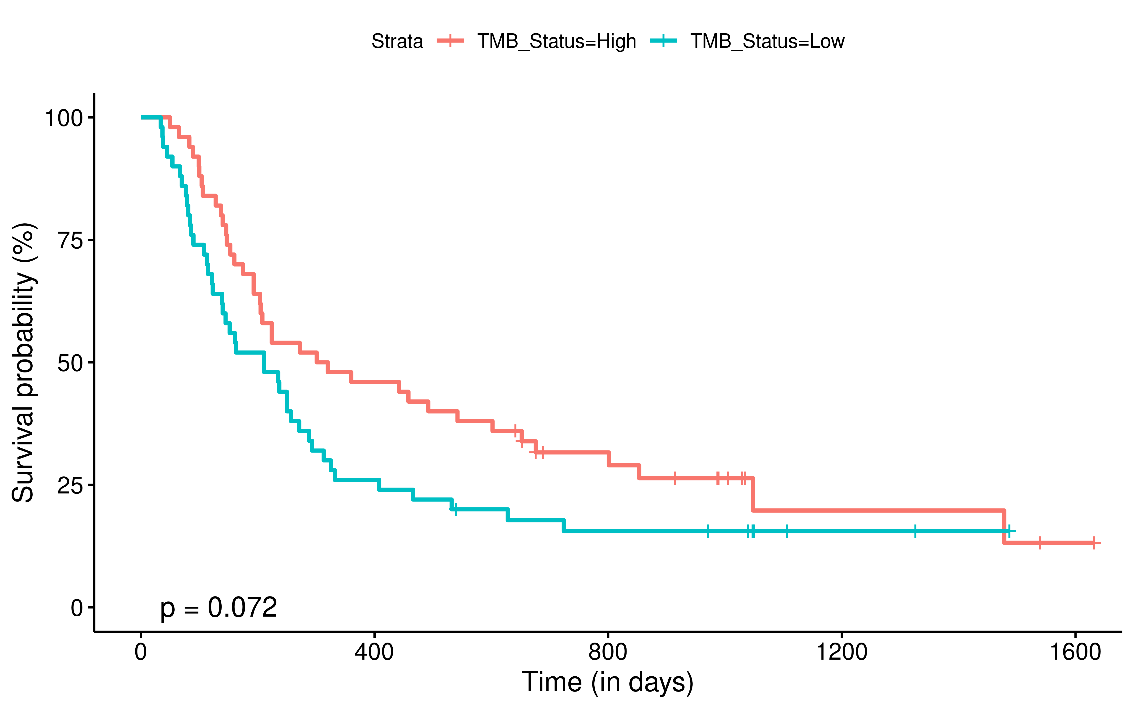
# effect of TIGS status on survival
fit2 <- survfit(Surv(overall_survival, dead == 1) ~ TIGS_Status, data = info_VanAllen3)
ggsurvplot(fit2, data = info_VanAllen3, pval = TRUE, fun = "pct", xlab = "Time (in days)")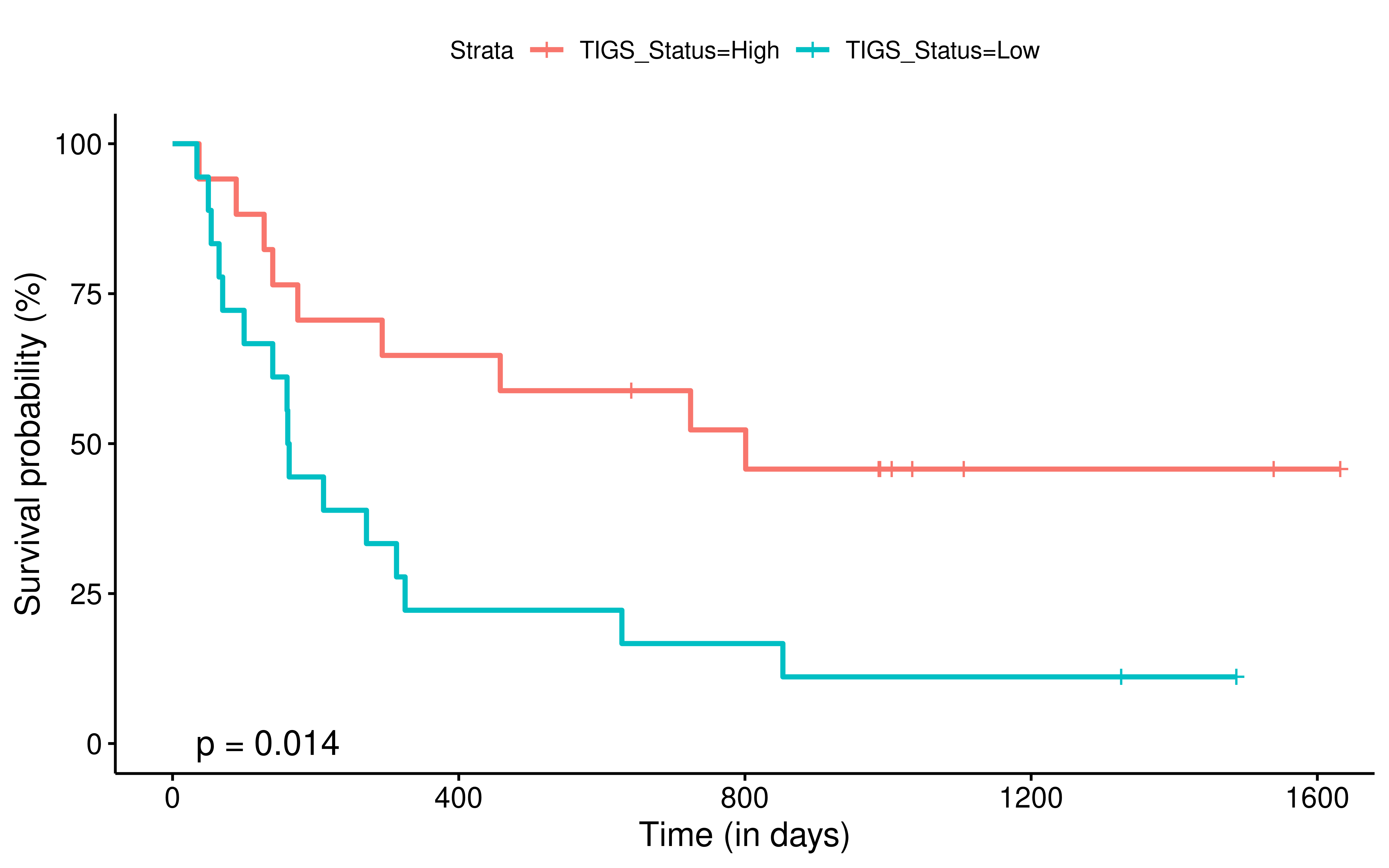
# effect of APS status on survival
fit3 <- survfit(Surv(overall_survival, dead == 1) ~ APS_Status, data = info_VanAllen3)
ggsurvplot(fit3,
  data = info_VanAllen3, pval = TRUE, fun = "pct",
  xlab = "Time (in days)"
)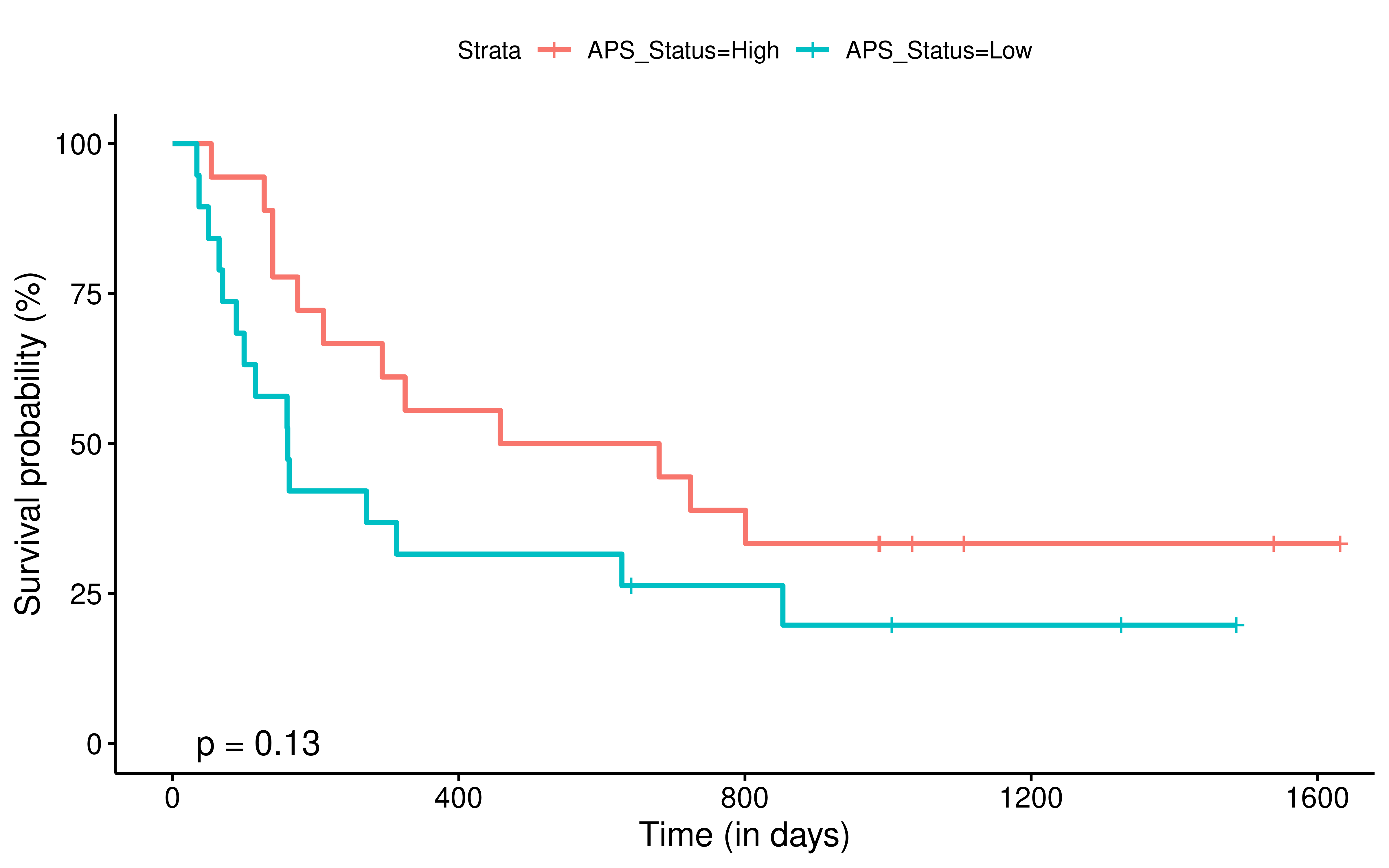
# effect of TIDE status on survival
fit4 <- survfit(Surv(overall_survival, dead == 1) ~ TIDE_Status, data = info_VanAllen3)
ggsurvplot(fit4, data = info_VanAllen3, pval = TRUE, fun = "pct", xlab = "Time (in days)")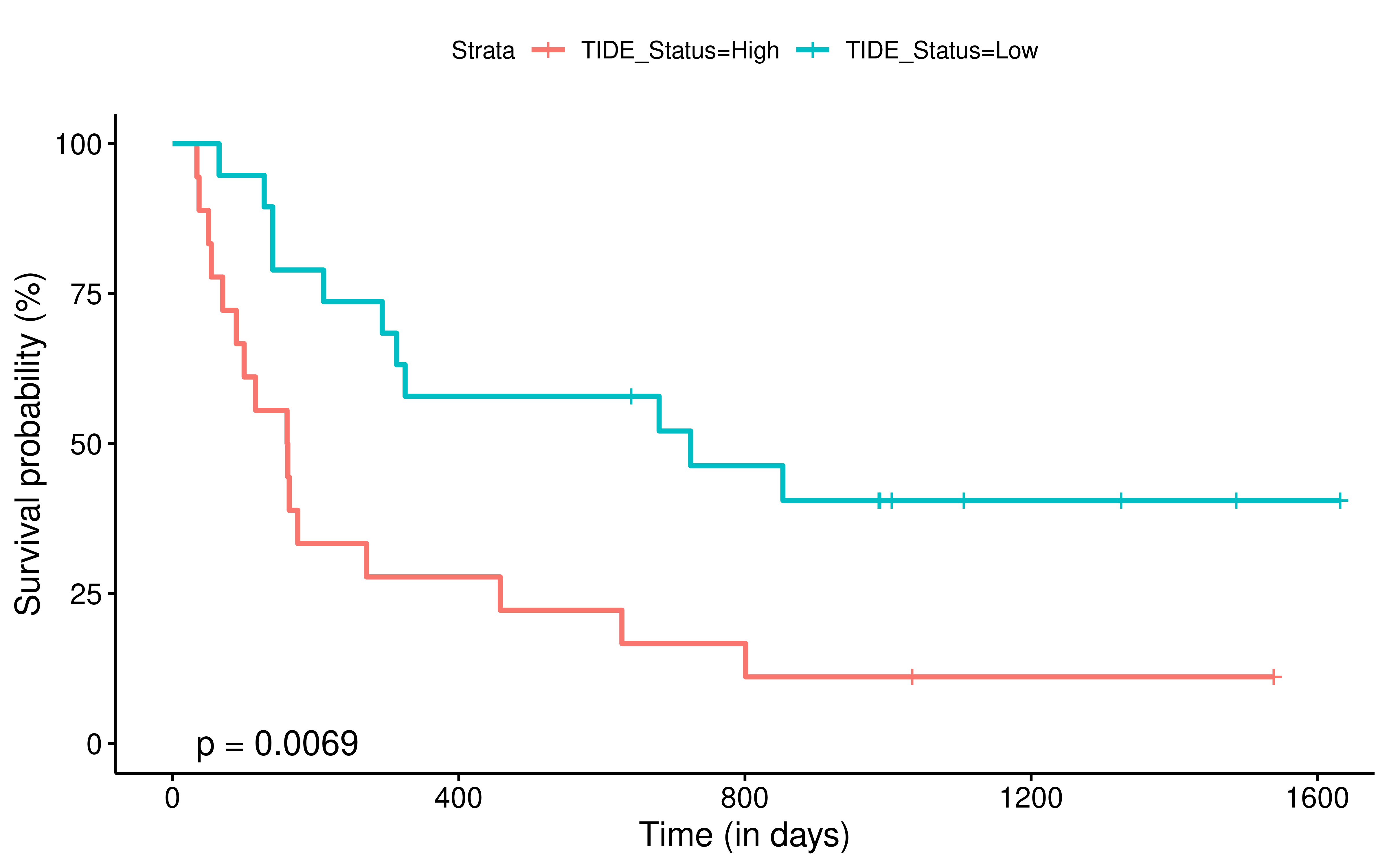
#----------------------
# Snyder 2017

# Cox model

# Cox result of TMB
coxph(Surv(os, event) ~ nTMB, data = info_Snyder)
#> Call:
#> coxph(formula = Surv(os, event) ~ nTMB, data = info_Snyder)
#>
#>       coef exp(coef) se(coef)  z   p
#> nTMB -0.02      0.98     0.02 -1 0.3
#>
#> Likelihood ratio test=1  on 1 df, p=0.3
#> n= 22, number of events= 14
#>    (6 observations deleted due to missingness)

# Cox result of APS
coxph(Surv(os, event) ~ APS, data = info_Snyder)
#> Call:
#> coxph(formula = Surv(os, event) ~ APS, data = info_Snyder)
#>
#>     coef exp(coef) se(coef)    z   p
#> APS -1.0       0.4      1.1 -0.9 0.4
#>
#> Likelihood ratio test=0.8  on 1 df, p=0.4
#> n= 25, number of events= 17
#>    (3 observations deleted due to missingness)

# Cox result of TIGS
coxph(Surv(os, event) ~ TIGS, data = info_Snyder)
#> Call:
#> coxph(formula = Surv(os, event) ~ TIGS, data = info_Snyder)
#>
#>      coef exp(coef) se(coef)  z   p
#> TIGS -0.5       0.6      0.3 -1 0.2
#>
#> Likelihood ratio test=2  on 1 df, p=0.1
#> n= 22, number of events= 14
#>    (6 observations deleted due to missingness)

# Cox result of TIDE
coxph(Surv(os, event) ~ TIDE, data = info_Snyder)
#> Call:
#> coxph(formula = Surv(os, event) ~ TIDE, data = info_Snyder)
#>
#>      coef exp(coef) se(coef) z   p
#> TIDE    1         3        1 1 0.2
#>
#> Likelihood ratio test=1  on 1 df, p=0.2
#> n= 25, number of events= 17
#>    (3 observations deleted due to missingness)


info_Snyder %>%
  mutate(
    APS_Status = ifelse(APS > median(APS, na.rm = TRUE), "High",
      ifelse(is.na(APS), NA, "Low")
    ),
    # We reverse TIDE (do TIDE=-TIDE) in previous step
    # so here, we need to change the order
    TIDE_Status = ifelse(TIDE < median(TIDE, na.rm = TRUE), "High",
      ifelse(is.na(TIDE), NA, "Low")
    ),
    TMB_Status = ifelse(nTMB > median(nTMB, na.rm = TRUE), "High",
      ifelse(is.na(nTMB), NA, "Low")
    ),
    TIGS_Status = ifelse(TIGS > median(TIGS, na.rm = TRUE), "High",
      ifelse(is.na(TIGS), NA, "Low")
    )
  ) -> info_Snyder2

# effect of TMB status on survival
fit1 <- survfit(Surv(os, event) ~ TMB_Status, data = info_Snyder2)
ggsurvplot(fit1,
  data = info_Snyder2, pval = TRUE, fun = "pct",
  xlab = "Time (in days)"
)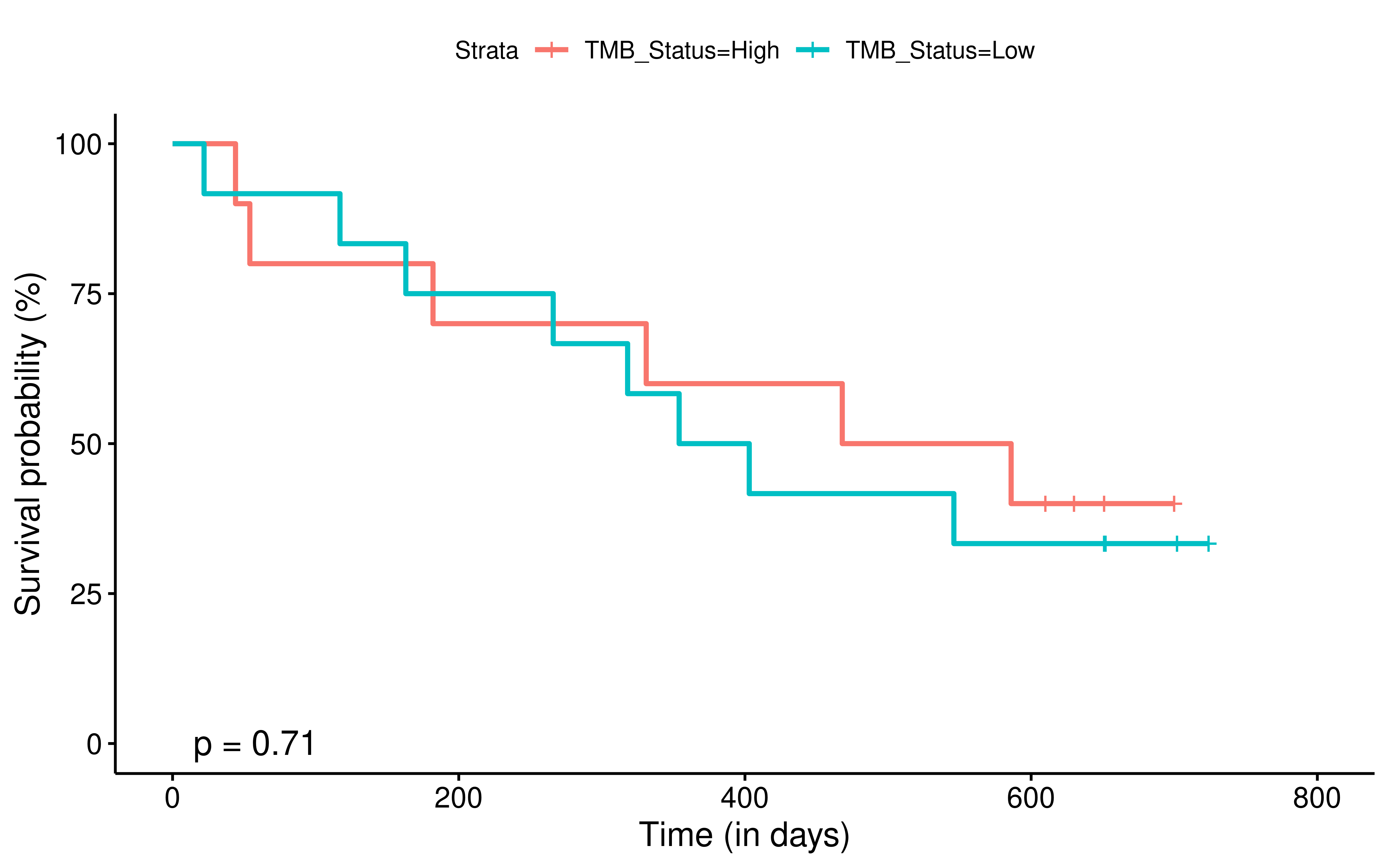
# effect of TIGS status on survival
fit2 <- survfit(Surv(os, event) ~ TIGS_Status, data = info_Snyder2)
ggsurvplot(fit2, data = info_Snyder2, pval = TRUE, fun = "pct", xlab = "Time (in days)")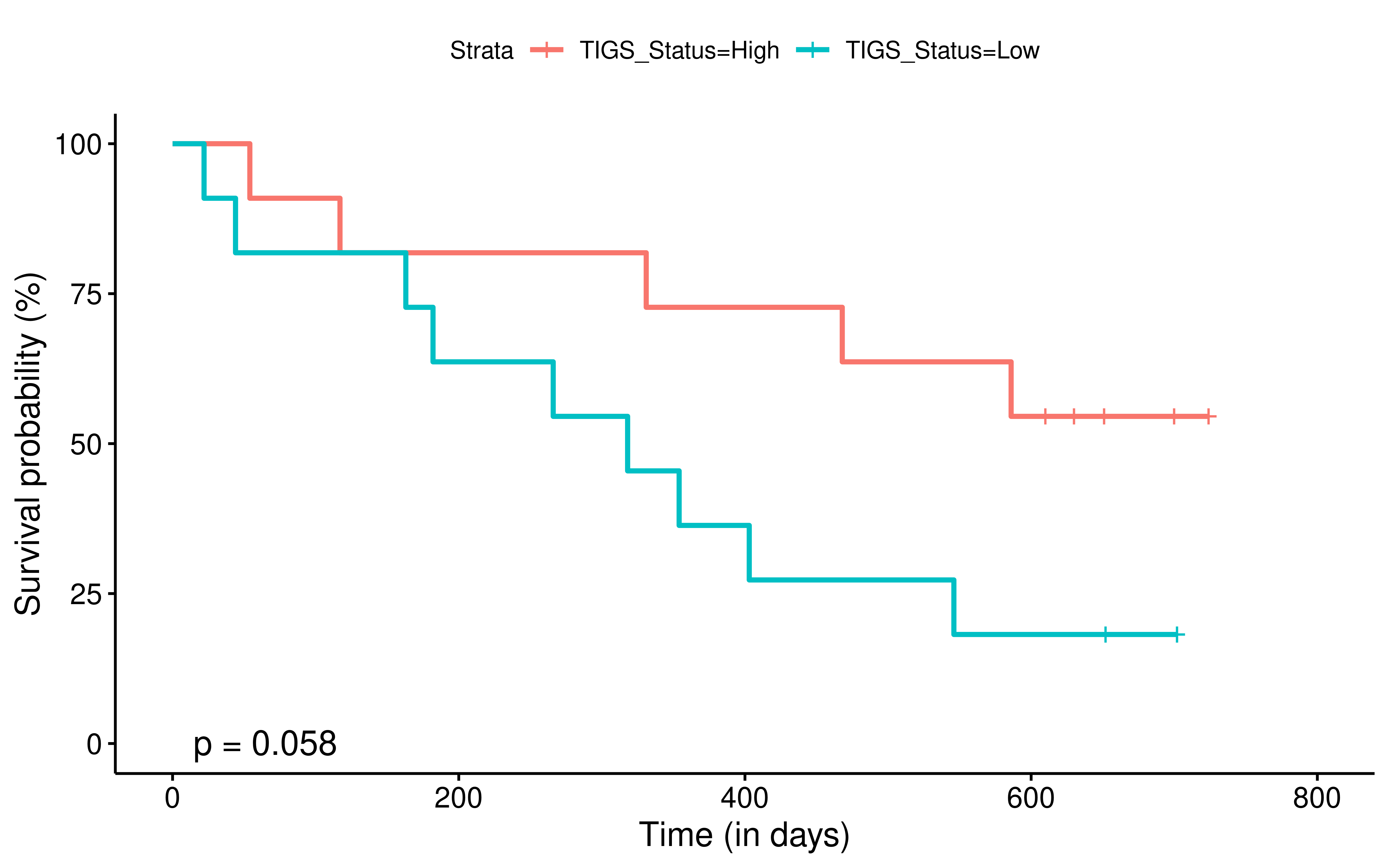
# effect of APS status on survival
fit3 <- survfit(Surv(os, event) ~ APS_Status, data = info_Snyder2)
ggsurvplot(fit3,
  data = info_Snyder2, pval = TRUE, fun = "pct",
  xlab = "Time (in days)"
)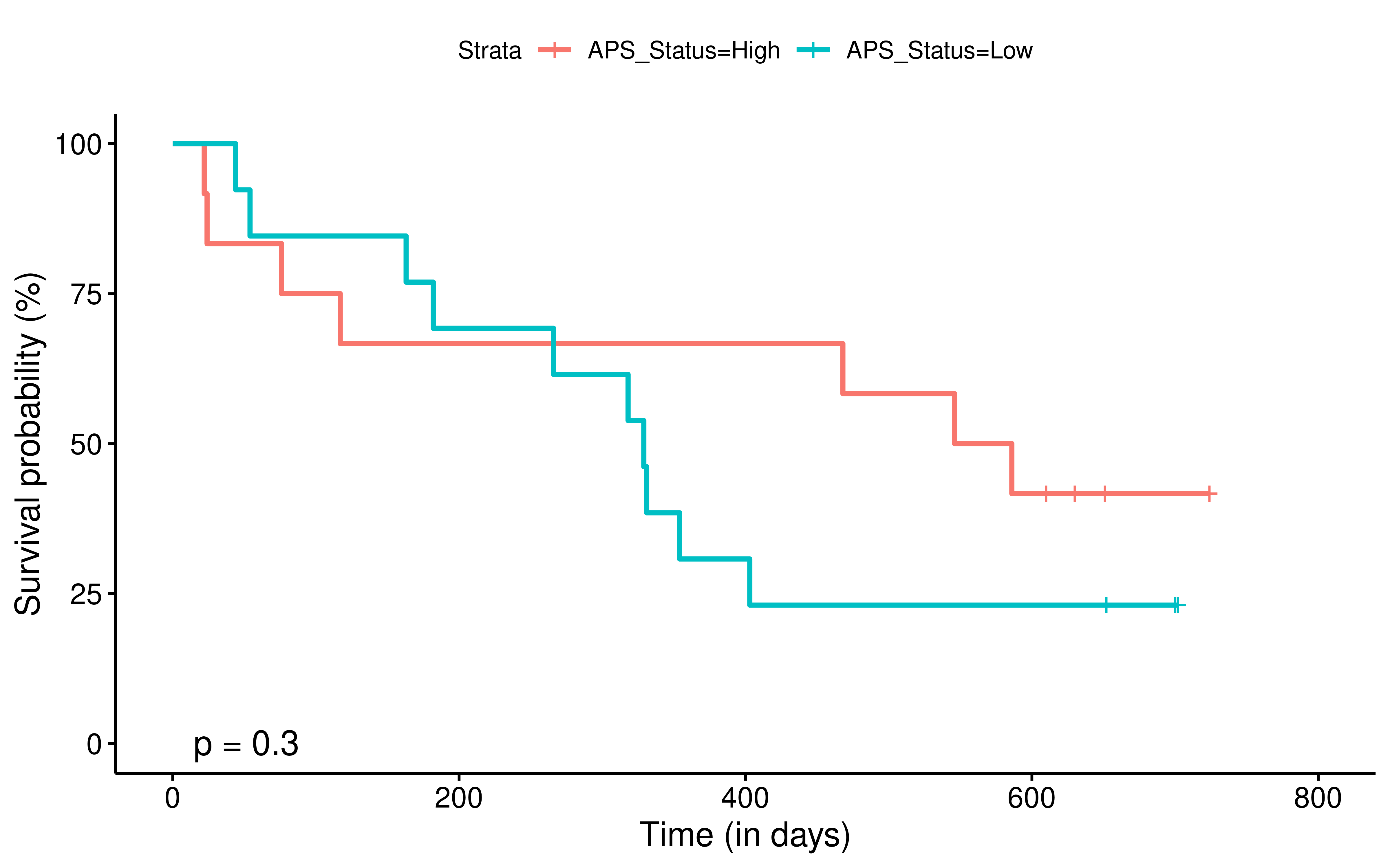
# effect of TIDE status on survival
fit4 <- survfit(Surv(os, event) ~ TIDE_Status, data = info_Snyder2)
ggsurvplot(fit4, data = info_Snyder2, pval = TRUE, fun = "pct", xlab = "Time (in days)")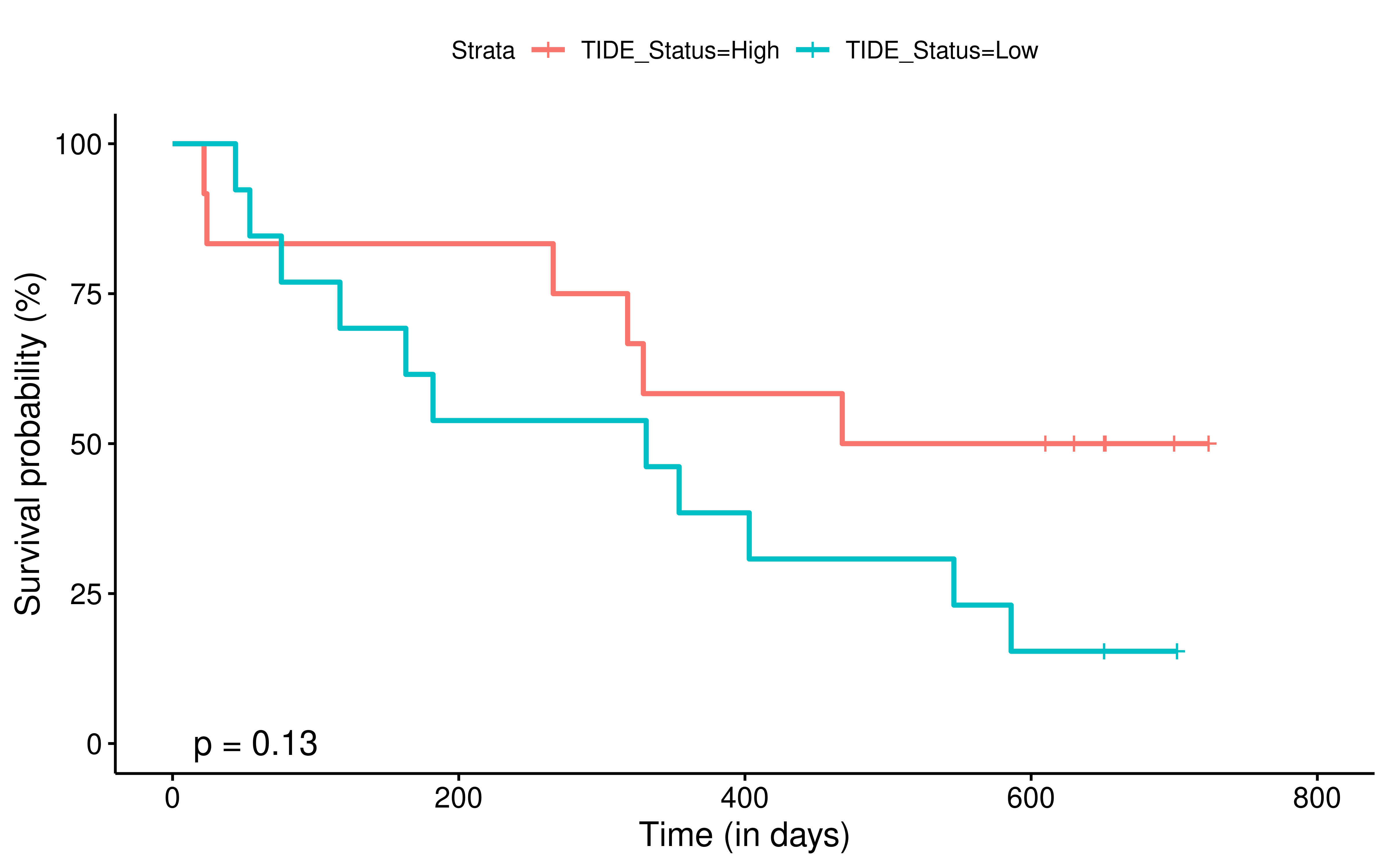
From comparison of cox results and K-M plots above, we can conclude that:
- TIGS is very robust, in all three datasets, “High group” all show statistically significant better survival than “Low group”.
- TIDE performs just so-so in Hugo 2016 dataset, very good in Van Allen 2015 dataset. But, it losts its power in Snyder 2017 dataset, patients with low TIDE value should have better survival but in this dataset patients with high TIDE value have better survival.
- Patients with High TMB or APS in three datasets all show trends of better survival but not statistically significant.
Next, we summary results (cox HR value and K-M fit) above for final visualization.
# summary cox result
cox_TMB <- list()
cox_APS <- list()
cox_TIGS <- list()
cox_TIDE <- list()

summary(coxph(Surv(OverallSurvival, VitalStatus == "Dead") ~ nTMB, data = info_hugo)) -> cox_TMB[[1]]
summary(coxph(Surv(OverallSurvival, VitalStatus == "Dead") ~ APS, data = info_hugo)) -> cox_APS[[1]]
summary(coxph(Surv(OverallSurvival, VitalStatus == "Dead") ~ TIGS, data = info_hugo)) -> cox_TIGS[[1]]
summary(coxph(Surv(OverallSurvival, VitalStatus == "Dead") ~ TIDE, data = info_hugo)) -> cox_TIDE[[1]]

summary(coxph(Surv(overall_survival, dead == 1) ~ nTMB, data = info_VanAllen)) -> cox_TMB[[2]]
summary(coxph(Surv(overall_survival, dead == 1) ~ APS, data = info_VanAllen)) -> cox_APS[[2]]
summary(coxph(Surv(overall_survival, dead == 1) ~ TIGS, data = info_VanAllen)) -> cox_TIGS[[2]]
summary(coxph(Surv(overall_survival, dead == 1) ~ TIDE, data = info_VanAllen)) -> cox_TIDE[[2]]

summary(coxph(Surv(os, event) ~ nTMB, data = info_Snyder)) -> cox_TMB[[3]]
summary(coxph(Surv(os, event) ~ APS, data = info_Snyder)) -> cox_APS[[3]]
summary(coxph(Surv(os, event) ~ TIGS, data = info_Snyder)) -> cox_TIGS[[3]]
summary(coxph(Surv(os, event) ~ TIDE, data = info_Snyder)) -> cox_TIDE[[3]]

cox_df <- tibble(
  Group = c(rep("Hugo2016", 4), rep("VanAllen2015", 4), rep("Snyder2017", 4)),
  Biomarker = rep(c("TMB", "APS", "TIGS", "TIDE"), 3),
  HR = c(
    as.numeric(cox_TMB[[1]]$conf.int[1]),
    as.numeric(cox_APS[[1]]$conf.int[1]),
    as.numeric(cox_TIGS[[1]]$conf.int[1]),
    as.numeric(cox_TIDE[[1]]$conf.int[1]),
    as.numeric(cox_TMB[[2]]$conf.int[1]),
    as.numeric(cox_APS[[2]]$conf.int[1]),
    as.numeric(cox_TIGS[[2]]$conf.int[1]),
    as.numeric(cox_TIDE[[2]]$conf.int[1]),
    as.numeric(cox_TMB[[3]]$conf.int[1]),
    as.numeric(cox_APS[[3]]$conf.int[1]),
    as.numeric(cox_TIGS[[3]]$conf.int[1]),
    as.numeric(cox_TIDE[[3]]$conf.int[1])
  ),
  Pvalue = c(
    as.numeric(cox_TMB[[1]]$logtest["pvalue"]),
    as.numeric(cox_APS[[1]]$logtest["pvalue"]),
    as.numeric(cox_TIGS[[1]]$logtest["pvalue"]),
    as.numeric(cox_TIDE[[1]]$logtest["pvalue"]),
    as.numeric(cox_TMB[[2]]$logtest["pvalue"]),
    as.numeric(cox_APS[[2]]$logtest["pvalue"]),
    as.numeric(cox_TIGS[[2]]$logtest["pvalue"]),
    as.numeric(cox_TIDE[[2]]$logtest["pvalue"]),
    as.numeric(cox_TMB[[3]]$logtest["pvalue"]),
    as.numeric(cox_APS[[3]]$logtest["pvalue"]),
    as.numeric(cox_TIGS[[3]]$logtest["pvalue"]),
    as.numeric(cox_TIDE[[3]]$logtest["pvalue"])
  )
)

# show summary data as table
DT::datatable(cox_df,
  options = list(scrollX = TRUE, keys = TRUE), rownames = FALSE,
  caption = "HR of biomarkers for response prediction in three ICB datasets"
)
# summary K-M fit
km_TMB <- list()
km_APS <- list()
km_TIGS <- list()
km_TIDE <- list()


km_TMB[["Hugo"]] <- survfit(Surv(OverallSurvival, VitalStatus == "Dead") ~ TMB_Status, data = info_hugo2)
km_TIGS[["Hugo"]] <- survfit(Surv(OverallSurvival, VitalStatus == "Dead") ~ TIGS_Status, data = info_hugo2)
km_APS[["Hugo"]] <- survfit(Surv(OverallSurvival, VitalStatus == "Dead") ~ APS_Status, data = info_hugo2)
km_TIDE[["Hugo"]] <- survfit(Surv(OverallSurvival, VitalStatus == "Dead") ~ TIDE_Status, data = info_hugo2)

km_TMB[["VanAllen"]] <- survfit(Surv(overall_survival, dead == 1) ~ TMB_Status, data = info_VanAllen3)
km_TIGS[["VanAllen"]] <- survfit(Surv(overall_survival, dead == 1) ~ TIGS_Status, data = info_VanAllen3)
km_APS[["VanAllen"]] <- survfit(Surv(overall_survival, dead == 1) ~ APS_Status, data = info_VanAllen3)
km_TIDE[["VanAllen"]] <- survfit(Surv(overall_survival, dead == 1) ~ TIDE_Status, data = info_VanAllen3)


km_TMB[["Snyder"]] <- survfit(Surv(os, event) ~ TMB_Status, data = info_Snyder2)
km_TIGS[["Snyder"]] <- survfit(Surv(os, event) ~ TIGS_Status, data = info_Snyder2)
km_APS[["Snyder"]] <- survfit(Surv(os, event) ~ APS_Status, data = info_Snyder2)
km_TIDE[["Snyder"]] <- survfit(Surv(os, event) ~ TIDE_Status, data = info_Snyder2)


km_fit <- list(TMB = km_TMB, APS = km_APS, TIGS = km_TIGS, TIDE = km_TIDE)

if (!file.exists("results/cox_km_result.RData")) {
  save(cox_df, km_fit, file = "results/cox_km_result.RData")
}
Visualization of comparison profile
This section we visualize comparsion profile, integrate analysis results of 3 immunotherapy datasets into a big figure.
# make sure these package are loaded
library(pROC)
# library(ggsci)
library(ggplot2)
suppressPackageStartupMessages(library(cowplot))
Integrate ROC curve.
theme_set(cowplot::theme_cowplot())

## -------- ROC

# Van Allen
p_roc_1 <- ggroc(list(TMB = van2015_roc$nTMB,
                      TIGS = van2015_roc$TIGS,
                      TIDE = van2015_roc$TIDE), legacy.axes = TRUE, aes = c("color", "linetype")) +
  scale_color_manual("", values = c("blue", "red", "black")) +
  scale_linetype_discrete("") +
  theme(legend.position = c(0.8, 0.4)) +
  geom_segment(aes(x=0, xend=1, y =0, yend=1), color = "grey", linetype = "dashed")
# Hugo
p_roc_2 <- ggroc(list(TMB = hugo2016_roc$nTMB,
                      TIGS = hugo2016_roc$TIGS,
                      TIDE = hugo2016_roc$TIDE), legacy.axes = TRUE, aes = c("color", "linetype")) +
  scale_color_manual("", values = c("blue", "red", "black")) +
  scale_linetype_discrete("") +
  theme(legend.position = c(0.8, 0.4)) +
  geom_segment(aes(x=0, xend=1, y =0, yend=1), color = "grey", linetype = "dashed")
# Snyder
p_roc_3 <- ggroc(list(TMB = snyder2017_roc$nTMB,
                      TIGS = snyder2017_roc$TIGS,
                      TIDE = snyder2017_roc$TIDE), legacy.axes = TRUE, aes = c("color", "linetype")) +
  scale_color_manual("", values = c("blue", "red", "black")) +
  scale_linetype_discrete("") +
  theme(legend.position = c(0.8, 0.4)) +
  geom_segment(aes(x=0, xend=1, y =0, yend=1), color = "grey", linetype = "dashed")

p_roc_4 <- ggroc(list(
  TIGS = van2015_roc$TIGS, APS = van2015_roc$APS, PDL1 = van2015_roc$PDL1,
  CD8 = van2015_roc$CD8, IFNG = van2015_roc$IFNG, IIS = van2015_roc$IIS,
  ISG.RS = van2015_roc$ISG.RS, IFNG.GS = van2015_roc$IFNG.GS), aes = c("color", "linetype"),
  legacy.axes = TRUE) +
  scale_color_discrete("") +
  scale_linetype_discrete("") +
  theme(legend.position = c(0.8, 0.4)) +
  geom_segment(aes(x=0, xend=1, y =0, yend=1), color = "grey", linetype = "dashed")

p_roc_5 <- ggroc(list(
  TIGS = hugo2016_roc$TIGS, APS = hugo2016_roc$APS, PDL1 = hugo2016_roc$PDL1,
  CD8 = hugo2016_roc$CD8, IFNG = hugo2016_roc$IFNG, IIS = hugo2016_roc$IIS,
  ISG.RS = hugo2016_roc$ISG.RS, IFNG.GS = hugo2016_roc$IFNG.GS), aes = c("color", "linetype"),
  legacy.axes = TRUE) +
  scale_color_discrete("") +
  scale_linetype_discrete("") +
  theme(legend.position = c(0.8, 0.4)) +
  geom_segment(aes(x=0, xend=1, y =0, yend=1), color = "grey", linetype = "dashed")

p_roc_6 <- ggroc(list(
  TIGS = snyder2017_roc$TIGS, APS = snyder2017_roc$APS, PDL1 = snyder2017_roc$PDL1,
  CD8 = snyder2017_roc$CD8, IFNG = snyder2017_roc$IFNG, IIS = snyder2017_roc$IIS,
  ISG.RS = snyder2017_roc$ISG.RS, IFNG.GS = snyder2017_roc$IFNG.GS), aes = c("color", "linetype"),
  legacy.axes = TRUE) +
  scale_color_discrete("") +
  scale_linetype_discrete("") +
  theme(legend.position = c(0.8, 0.4)) +
  geom_segment(aes(x=0, xend=1, y =0, yend=1), color = "grey", linetype = "dashed")


p_extra <- plot_grid(p_roc_4, p_roc_5, p_roc_6, nrow = 1)
save_plot(filename = "extra_roc_comparison.pdf", plot = p_extra, nrow = 1,
          ncol = 3, base_aspect_ratio = 1.5)
show_cols = c("APS", "APSr", "IIS", "TMB", "TIGS", "TIDE", "CD8", "PDL1", "IFNG", "IFNG.GS", "ISG.RS")
show_extcols = c("TIDE_comb_TMB", "APS7_Sig", "APS7_Sig_comb_TMB")
## -------- AUC values
auc_df_long <- auc_df %>%
dplyr::select(c(colnames(auc_df)[1:20], "APSr", "Group")) %>%
tidyr::gather(key = "biomarker", value = "auc", -Group)
# p_auc_1 =
auc_df_long$auc <- round(auc_df_long$auc, digits = 3)
# AUC for PHBR comes from result of code/PHBR_comparison_*.R
auc_df_long %>%
filter(Group == "VanAllen2015", biomarker %in% show_cols) %>%
ggplot(aes(x = biomarker, y = auc)) +
geom_bar(stat = "identity", fill = "lightblue") +
geom_text(aes(label = auc), hjust = 1) +
geom_hline(yintercept = 0.5, linetype = 2) +
ylim(0, 0.85) + ylab("AUC") + theme(axis.title.y = element_blank()) +
coord_flip() -> p_auc_1
auc_df_long %>%
filter(Group == "Hugo2016", biomarker %in% show_cols) %>%
ggplot(aes(x = biomarker, y = auc)) +
geom_bar(stat = "identity", fill = "lightblue") +
geom_text(aes(label = auc), hjust = 1) +
geom_hline(yintercept = 0.5, linetype = 2) +
ylim(0, 0.8) + ylab("AUC") + theme(axis.title.y = element_blank()) +
coord_flip() -> p_auc_2
auc_df_long %>%
filter(Group == "Snyder2017", biomarker %in% show_cols) %>%
ggplot(aes(x = biomarker, y = auc)) +
geom_bar(stat = "identity", fill = "lightblue") +
geom_text(aes(label = auc), hjust = 1) +
geom_hline(yintercept = 0.5, linetype = 2) +
ylim(0, 0.8) + ylab("AUC") + theme(axis.title.y = element_blank()) +
coord_flip() -> p_auc_3
auc_df_long %>%
filter(Group == "VanAllen2015", biomarker %in% show_extcols) %>%
add_row(Group="VanAllen2015", biomarker=c("PHBR_I", "PHBR_I_comb_TMB"), auc=c(0.57, 0.71)) %>%
ggplot(aes(x = biomarker, y = auc)) +
geom_bar(stat = "identity", fill = "lightblue") +
geom_text(aes(label = auc), hjust = 1) +
geom_hline(yintercept = 0.5, linetype = 2) +
ylim(0, 0.85) + ylab("AUC") + theme(axis.title.y = element_blank()) +
coord_flip() -> p_auc_ext1
auc_df_long %>%
filter(Group == "Hugo2016", biomarker %in% show_extcols) %>%
ggplot(aes(x = biomarker, y = auc)) +
geom_bar(stat = "identity", fill = "lightblue") +
geom_text(aes(label = auc), hjust = 1) +
geom_hline(yintercept = 0.5, linetype = 2) +
ylim(0, 0.8) + ylab("AUC") + theme(axis.title.y = element_blank()) +
coord_flip() -> p_auc_ext2
auc_df_long %>%
filter(Group == "Snyder2017", biomarker %in% show_extcols) %>%
add_row(Group="Snyder2017", biomarker=c("PHBR_I", "PHBR_I_comb_TMB"), auc=c(0.68, 0.52)) %>%
ggplot(aes(x = biomarker, y = auc)) +
geom_bar(stat = "identity", fill = "lightblue") +
geom_text(aes(label = auc), hjust = 1) +
geom_hline(yintercept = 0.5, linetype = 2) +
ylim(0, 0.8) + ylab("AUC") + theme(axis.title.y = element_blank()) +
coord_flip() -> p_auc_ext3auc_ext = cowplot::plot_grid(p_auc_ext1 + ggtitle("Van Allen et al 2015"),
p_auc_ext2 + ggtitle("Hugo et al 2016"),
p_auc_ext3 + ggtitle("Snyder et al 2017"), nrow = 1)
ggsave("extra_auc.pdf", auc_ext, width = 12, height = 2.5)#--- KM-plots
p_surv_APS <- list()
p_surv_TMB <- list()
p_surv_TIGS <- list()
p_surv_TIDE <- list()
p_surv_APS[[1]] <- ggsurvplot(km_APS$VanAllen,
pval = TRUE, fun = "pct",
xlab = "Time (in days)", palette = c("red", "blue"),
legend = c(0.8, 0.9), legend.title = element_blank(), legend.labs = c("APS High", "APS Low")
)
p_surv_APS[[2]] <- ggsurvplot(km_APS$Hugo,
pval = TRUE, fun = "pct",
xlab = "Time (in days)", palette = c("red", "blue"),
legend = c(0.8, 0.9), legend.title = element_blank(), legend.labs = c("APS High", "APS Low")
)
p_surv_APS[[3]] <- ggsurvplot(km_APS$Snyder,
pval = TRUE, fun = "pct",
xlab = "Time (in days)", palette = c("red", "blue"),
legend = c(0.8, 0.9), legend.title = element_blank(), legend.labs = c("APS High", "APS Low")
)
p_surv_TMB[[1]] <- ggsurvplot(km_TMB$VanAllen,
pval = TRUE, fun = "pct",
xlab = "Time (in days)", palette = c("red", "blue"),
legend = c(0.8, 0.9), legend.title = element_blank(), legend.labs = c("TMB High", "TMB Low")
)
p_surv_TMB[[2]] <- ggsurvplot(km_TMB$Hugo,
pval = TRUE, fun = "pct",
xlab = "Time (in days)", palette = c("red", "blue"),
legend = c(0.8, 0.9), legend.title = element_blank(), legend.labs = c("TMB High", "TMB Low")
)
p_surv_TMB[[3]] <- ggsurvplot(km_TMB$Snyder,
pval = TRUE, fun = "pct",
xlab = "Time (in days)", palette = c("red", "blue"),
legend = c(0.8, 0.9), legend.title = element_blank(), legend.labs = c("TMB High", "TMB Low")
)
p_surv_TIGS[[1]] <- ggsurvplot(km_TIGS$VanAllen,
pval = TRUE, fun = "pct",
xlab = "Time (in days)", palette = c("red", "blue"),
legend = c(0.8, 0.9), legend.title = element_blank(), legend.labs = c("TIGS High", "TIGS Low")
)
p_surv_TIGS[[2]] <- ggsurvplot(km_TIGS$Hugo,
pval = TRUE, fun = "pct",
xlab = "Time (in days)", palette = c("red", "blue"),
legend = c(0.8, 0.4), legend.title = element_blank(), legend.labs = c("TIGS High", "TIGS Low")
)
p_surv_TIGS[[3]] <- ggsurvplot(km_TIGS$Snyder,
pval = TRUE, fun = "pct",
xlab = "Time (in days)", palette = c("red", "blue"),
legend = c(0.8, 0.9), legend.title = element_blank(), legend.labs = c("TIGS High", "TIGS Low")
)
p_surv_TIDE[[1]] <- ggsurvplot(km_TIDE$VanAllen,
pval = TRUE, fun = "pct",
xlab = "Time (in days)", palette = c("red", "blue"),
legend = c(0.8, 0.9), legend.title = element_blank(), legend.labs = c("TIDE High", "TIDE Low")
)
p_surv_TIDE[[2]] <- ggsurvplot(km_TIDE$Hugo,
pval = TRUE, fun = "pct",
xlab = "Time (in days)", palette = c("red", "blue"),
legend = c(0.8, 0.9), legend.title = element_blank(), legend.labs = c("TIDE High", "TIDE Low")
)
p_surv_TIDE[[3]] <- ggsurvplot(km_TIDE$Snyder,
pval = TRUE, fun = "pct",
xlab = "Time (in days)", palette = c("red", "blue"),
legend = c(0.8, 0.9), legend.title = element_blank(), legend.labs = c("TIDE High", "TIDE Low")
)
p_aps <- plot_grid(plotlist = lapply(p_surv_APS, function(x) x$plot), ncol = 3)
save_plot(filename = "aps_kmplot.pdf", plot = p_aps, ncol = 3, base_aspect_ratio = 1.3)
# ggpar(p , font.legend = c(12, "bold", "black"))plot_list = list(
p_roc_1, p_roc_2, p_roc_3,
p_auc_1, p_auc_2, p_auc_3,
p_surv_TMB[[1]]$plot, p_surv_TMB[[2]]$plot, p_surv_TMB[[3]]$plot,
p_surv_TIGS[[1]]$plot, p_surv_TIGS[[2]]$plot, p_surv_TIGS[[3]]$plot,
p_surv_TIDE[[1]]$plot, p_surv_TIDE[[2]]$plot, p_surv_TIDE[[3]]$plot
)
# plot_list <- list(
# p_roc_1, p_auc_1, p_surv_TMB[[1]]$plot, p_surv_TIGS[[1]]$plot, p_surv_TIDE[[1]]$plot,
# p_roc_2, p_auc_2, p_surv_TMB[[2]]$plot, p_surv_TIGS[[2]]$plot, p_surv_TIDE[[2]]$plot,
# p_roc_3, p_auc_3, p_surv_TMB[[3]]$plot, p_surv_TIGS[[3]]$plot, p_surv_TIDE[[3]]$plot
# )
# plot_grid(p_roc_1, p_roc_2, p_roc_3,
# p_auc_1, p_auc_2, p_auc_3,
# p_surv_TMB[[1]]$plot, p_surv_TMB[[2]]$plot, p_surv_TMB[[3]]$plot,
# p_surv_TIGS[[1]]$plot, p_surv_TIGS[[2]]$plot, p_surv_TIGS[[3]]$plot,
# p_surv_TIDE[[1]]$plot, p_surv_TIDE[[2]]$plot, p_surv_TIDE[[3]]$plot, nrow = 3, ncol=5,
# align = "vh")
plot_res <- plot_grid(
plotlist = plot_list, nrow = 5, ncol = 3
)
save_plot("comp_profile.png", plot_res, nrow = 5, ncol = 3)
knitr::include_graphics("comp_profile.png")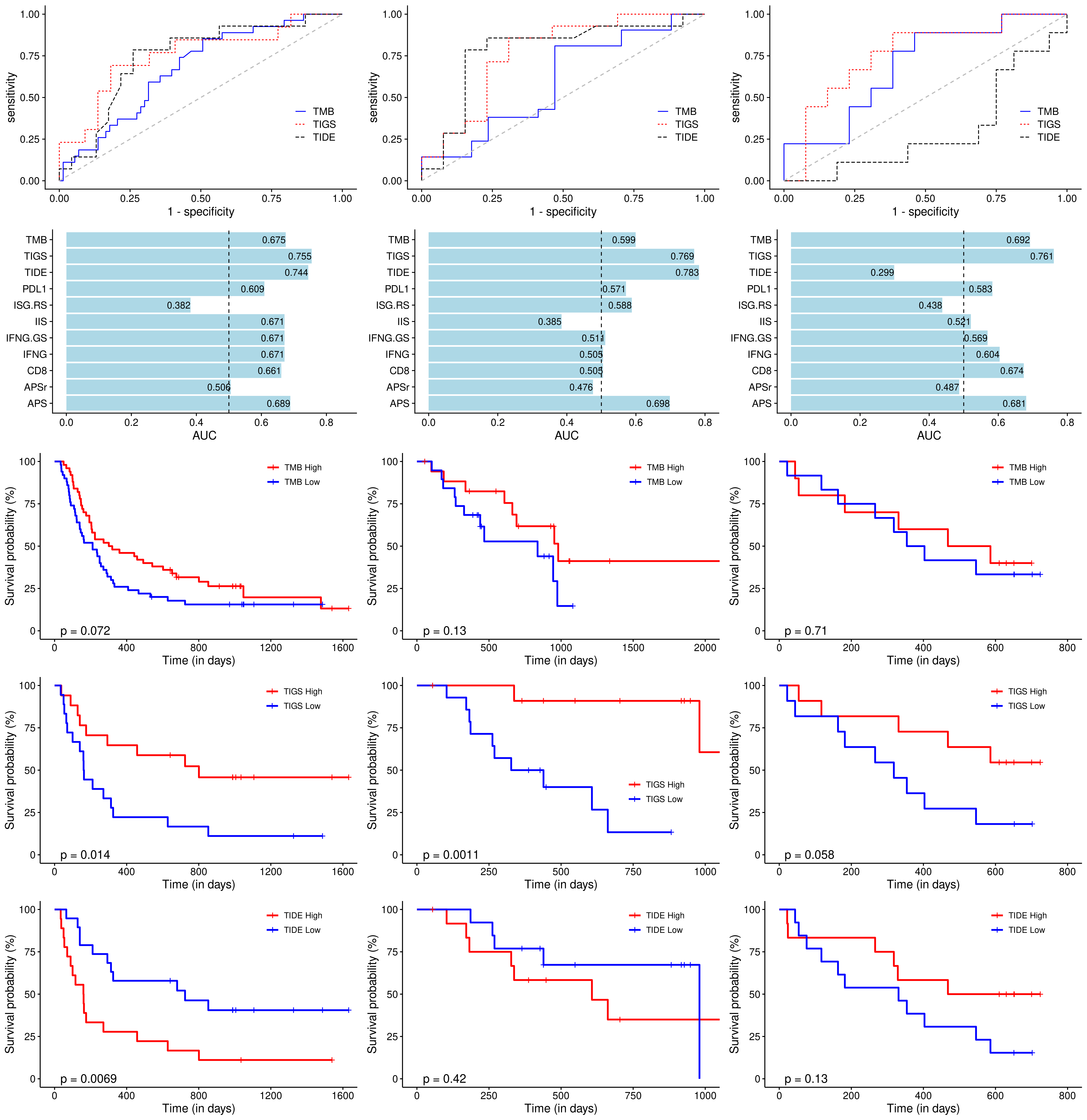
Save as pdf for publication.
Session info
sessionInfo()
#> R version 3.6.0 (2019-04-26)
#> Platform: x86_64-pc-linux-gnu (64-bit)
#> Running under: CentOS Linux 7 (Core)
#>
#> Matrix products: default
#> BLAS:   /home/public/R/R-base/lib64/R/lib/libRblas.so
#> LAPACK: /home/public/R/R-base/lib64/R/lib/libRlapack.so
#>
#> locale:
#>  [1] LC_CTYPE=en_US.UTF-8       LC_NUMERIC=C
#>  [3] LC_TIME=en_US.UTF-8        LC_COLLATE=en_US.UTF-8
#>  [5] LC_MONETARY=en_US.UTF-8    LC_MESSAGES=en_US.UTF-8
#>  [7] LC_PAPER=en_US.UTF-8       LC_NAME=C
#>  [9] LC_ADDRESS=C               LC_TELEPHONE=C
#> [11] LC_MEASUREMENT=en_US.UTF-8 LC_IDENTIFICATION=C
#>
#> attached base packages:
#> [1] grid      stats     graphics  grDevices utils     datasets  methods
#> [8] base
#>
#> other attached packages:
#>  [1] cowplot_1.0.0       survminer_0.4.6     pROC_1.15.3
#>  [4] ggrepel_0.8.1       forestplot_1.9      checkmate_1.9.4
#>  [7] survival_3.1-7      ggpubr_0.2.3        magrittr_1.5
#> [10] scales_1.0.0        corrplot_0.84       pheatmap_1.0.12
#> [13] forcats_0.4.0       stringr_1.4.0       purrr_0.3.3
#> [16] tidyr_1.0.0         tibble_2.1.3        ggplot2_3.2.1
#> [19] tidyverse_1.2.1     readr_1.3.1         dplyr_0.8.3
#> [22] UCSCXenaTools_1.2.7 rmdformats_0.3.5    knitr_1.26
#> [25] pacman_0.5.1
#>
#> loaded via a namespace (and not attached):
#>  [1] utf8_1.1.4             questionr_0.7.0        R.utils_2.9.0
#>  [4] tidyselect_0.2.5       lme4_1.1-21            robust_0.4-18.1
#>  [7] htmlwidgets_1.5.1      munsell_0.5.0          codetools_0.2-16
#> [10] DT_0.10                future_1.15.0          miniUI_0.1.1.1
#> [13] withr_2.1.2            Brobdingnag_1.2-6      metaBMA_0.6.2
#> [16] colorspace_1.4-1       highr_0.8              rstudioapi_0.10
#> [19] stats4_3.6.0           DescTools_0.99.30      robustbase_0.93-5
#> [22] rcompanion_2.3.7       ggsignif_0.6.0         listenv_0.7.0
#> [25] labeling_0.3           emmeans_1.4.2          rstan_2.19.2
#> [28] KMsurv_0.1-5           mnormt_1.5-5           MCMCpack_1.4-4
#> [31] bridgesampling_0.7-2   coda_0.19-3            vctrs_0.2.0
#> [34] generics_0.0.2         TH.data_1.0-10         metafor_2.1-0
#> [37] xfun_0.11              R6_2.4.0               BayesFactor_0.9.12-4.2
#> [40] reshape_0.8.8          logspline_2.1.15       assertthat_0.2.1
#> [43] promises_1.1.0         multcomp_1.4-10        ggExtra_0.9
#> [46] gtable_0.3.0           multcompView_0.1-7     globals_0.12.4
#> [49] processx_3.4.1         mcmc_0.9-6             sandwich_2.5-1
#> [52] rlang_0.4.1            MatrixModels_0.4-1     EMT_1.1
#> [55] zeallot_0.1.0          splines_3.6.0          TMB_1.7.15
#> [58] lazyeval_0.2.2         broom_0.5.2            inline_0.3.15
#> [61] abind_1.4-5            yaml_2.2.0             reshape2_1.4.3
#> [64] modelr_0.1.5           crosstalk_1.0.0        backports_1.1.5
#> [67] httpuv_1.5.2           tools_3.6.0            bookdown_0.15
#> [70] psych_1.8.12           ellipsis_0.3.0         RColorBrewer_1.1-2
#> [73] WRS2_1.0-0             ez_4.4-0               Rcpp_1.0.3
#>  [ reached getOption("max.print") -- omitted 100 entries ]
Supplementary analyses
Random selection of APM genes or IIS genes
TCGA contains about 10,000 patients with RNASeq data, it is hard to simulate GSVA serveral times with whole data (too much computation), thus we using a sampling strategy as following:
- randomly select RNAseq data from 500 patients.
- calculate GSVA score
- calculate once from right genes.
- randomly select genes (10 times) and run GSVA.
- calculate spearman correlation coefficient for normal APS and normal IIS, random APS and normal IIS, normal APS and random IIS, respectively. The latter two have ten values, we use their mean.
- repeat the process 100 times.
The GSVA score calculation is implemented by script code/random_simulation.R (this will take much time to finish). Next we calculate correlation using following commands.
source("../code/functions.R")
cor_res <- data.frame(stringsAsFactors = FALSE)
for (i in 1:100) {
  normal <- normal_res[[i]][[1]]
  normal <- calc_TisIIs(normal)

  r1 <- as.numeric(cor.test(normal$APM, normal$IIS, method = "spearman")$estimate)

  r2 <- c() # normal APM, random IIS
  r3 <- c() # random APM, normal IIS
  for (j in 1:10) {
    random <- random_res[[i]][[j]][[1]]
    tryCatch({
      random <- calc_TisIIs(random)
      r_random1 <- as.numeric(cor.test(normal$APM, random$IIS, method = "spearman")$estimate)
      r2 <- c(r2, r_random1)
      r_random2 <- as.numeric(cor.test(random$APM, normal$IIS, method = "spearman")$estimate)
      r3 <- c(r3, r_random2)
    },
    error = function(e) {
      NA
    }
    )
  }
  r2 <- mean(r2, na.rm = TRUE)
  r3 <- mean(r3, na.rm = TRUE)
  cor_res <- rbind(cor_res, c(r1, r2, r3))
}

colnames(cor_res) <- c("normal", "random_IIS", "random_APS")

write_tsv(cor_res, "results/randomGSVA.tsv")
Now, we plot spearman correlation efficient of 3 types.
library(tidyverse)
library(cowplot)
cor_res <- read_tsv("results/randomGSVA.tsv", col_types = cols())

cor_res_long <- gather(cor_res, key = "Type", value = "SpearmanCoeff")
cor_res_long$Type <- factor(cor_res_long$Type)

p <- ggplot(cor_res_long, aes(x = SpearmanCoeff, color = Type)) +
  stat_density(geom = "line") +
  xlab("Spearman correlation coefficient") + ylab("Density") +
  guides(color = guide_legend(title = NULL)) +
  scale_color_discrete(labels = c("r(APS, IIS)", "r(APSr, IIS)", "r(APS, IISr"))
p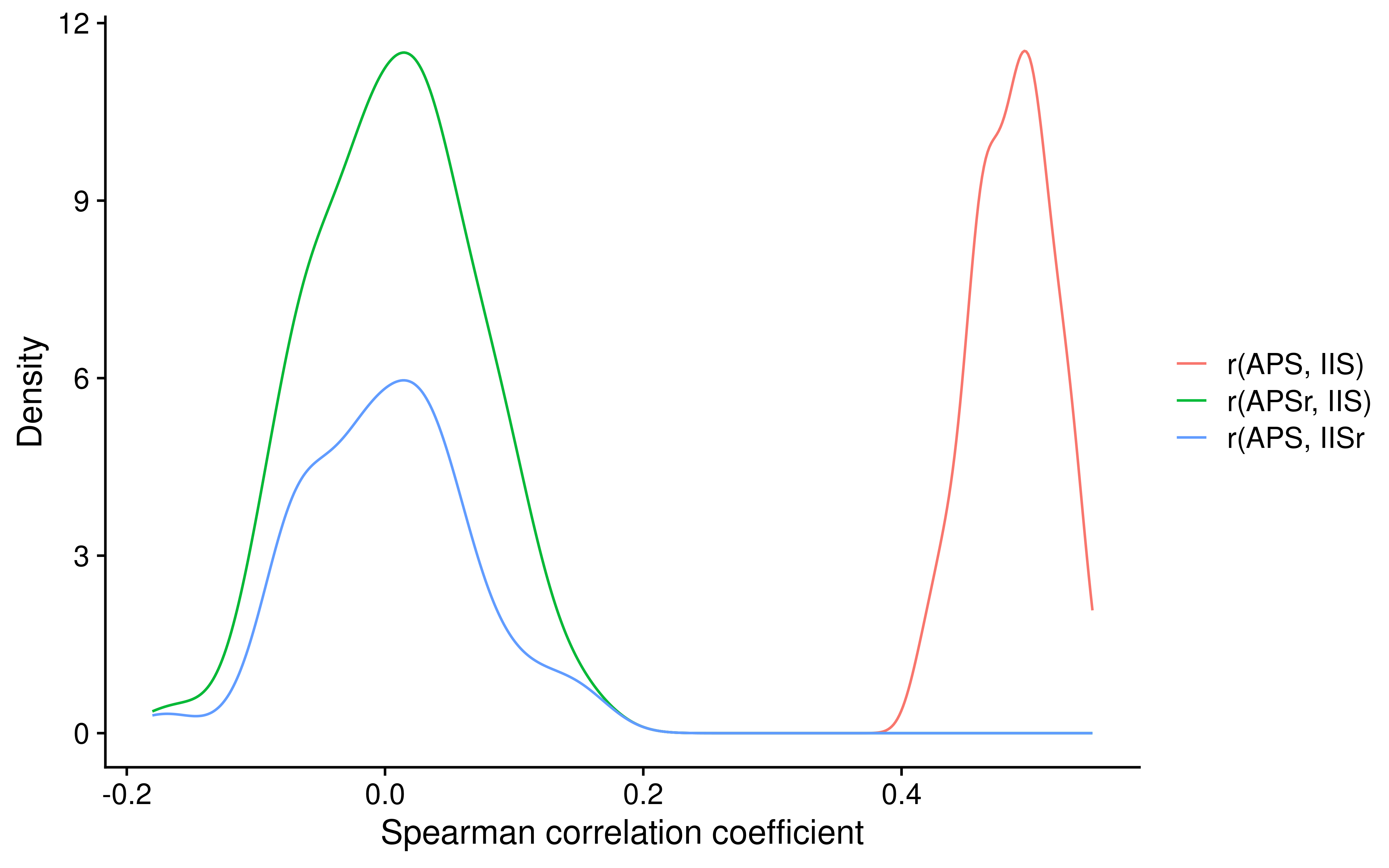
We can clearly see that if we change gene list for APS or IIS calculation, the strong positive correlation between APS and IIS will no longer exist.
Explore correlation between ORR and TIGS from TCGA data
A reviewer commented on our analysis which showed in section “TIGS definition and performance”:
it appears that the authors lumped together data from different data sets (e.g. reference 26 for tumor mutational burden and TCGA data for expression)
This analysis we adopted same idea from Tumor Mutational Burden and Response Rate to PD-1 inhibition. To further check reliability of this analysis, here we use gene expression and TMB data from TCGA and ORR data from clinical literatures.
Firstly we load TCGA data and calculate TIGS score.
library(dplyr)
load("results/TCGA_ALL.RData")

tcga_all <- tcga_all %>%
  mutate(
    nAPM = (APM - min(APM, na.rm = TRUE)) / (max(APM, na.rm = TRUE) - min(APM, na.rm = TRUE)),
    nTMB = TMB_NonsynVariants / 38,
    TIGS = log(nTMB + 1) * nAPM
  )
Next we calculate median of APS, TMB, TIGS and their corresponding sample counts for each tumor type.
tcga_tigs <- tcga_all %>%
  dplyr::filter(!is.na(Project)) %>%
  group_by(Project) %>%
  summarise(
    Patients_TIGS = sum(!is.na(TIGS)), TIGS = median(TIGS, na.rm = TRUE),
    Patients_APS = sum(!is.na(nAPM)), APS = median(nAPM, na.rm = TRUE),
    Patients_TMB = sum(!is.na(nTMB)), TMB = median(nTMB, na.rm = TRUE)
  )
DT::datatable(tcga_tigs)
We then save this data and merge them with ORR data according to corresponding tumor types.
After merging data, we load data into R.
tcga_orr <- readr:::read_csv("results/TCGA_TIGS_byProject2.csv")
#> Parsed with column specification:
#> cols(
#>   Project = col_character(),
#>   Patients_TIGS = col_double(),
#>   TIGS = col_double(),
#>   Patients_APS = col_double(),
#>   APS = col_double(),
#>   Patients_TMB = col_double(),
#>   TMB = col_double(),
#>   Patients_ORR = col_double(),
#>   ORR = col_double(),
#>   Long_Name = col_character()
#> )
Now we plot figures.
APS
ggplot(filter(tcga_orr, !is.na(ORR)), aes(x = APS, y = ORR)) +
  geom_point(aes(color = Patients_APS, size = Patients_ORR)) +
  geom_smooth(method = "lm", se = T) +
  geom_text_repel(aes(label = Project), size = 3) +
  labs(
    x = "Median Normalized APM Score ", y = "Objective Response Rate (%)",
    size = "Objective Response Rate\n(no. of patients evaluated)",
    color = "APM Score\n(no. of tumor analyzed)"
  ) +
  scale_size_continuous(breaks = c(50, 100, 500, 1000)) +
  scale_color_gradientn(
    colours = RColorBrewer::brewer.pal(5, name = "OrRd")[-1],
    breaks = c(50, 200, 500, 1000)
  ) +
  theme_bw() +
  guides(
    color = guide_colorbar(order = 1)
  )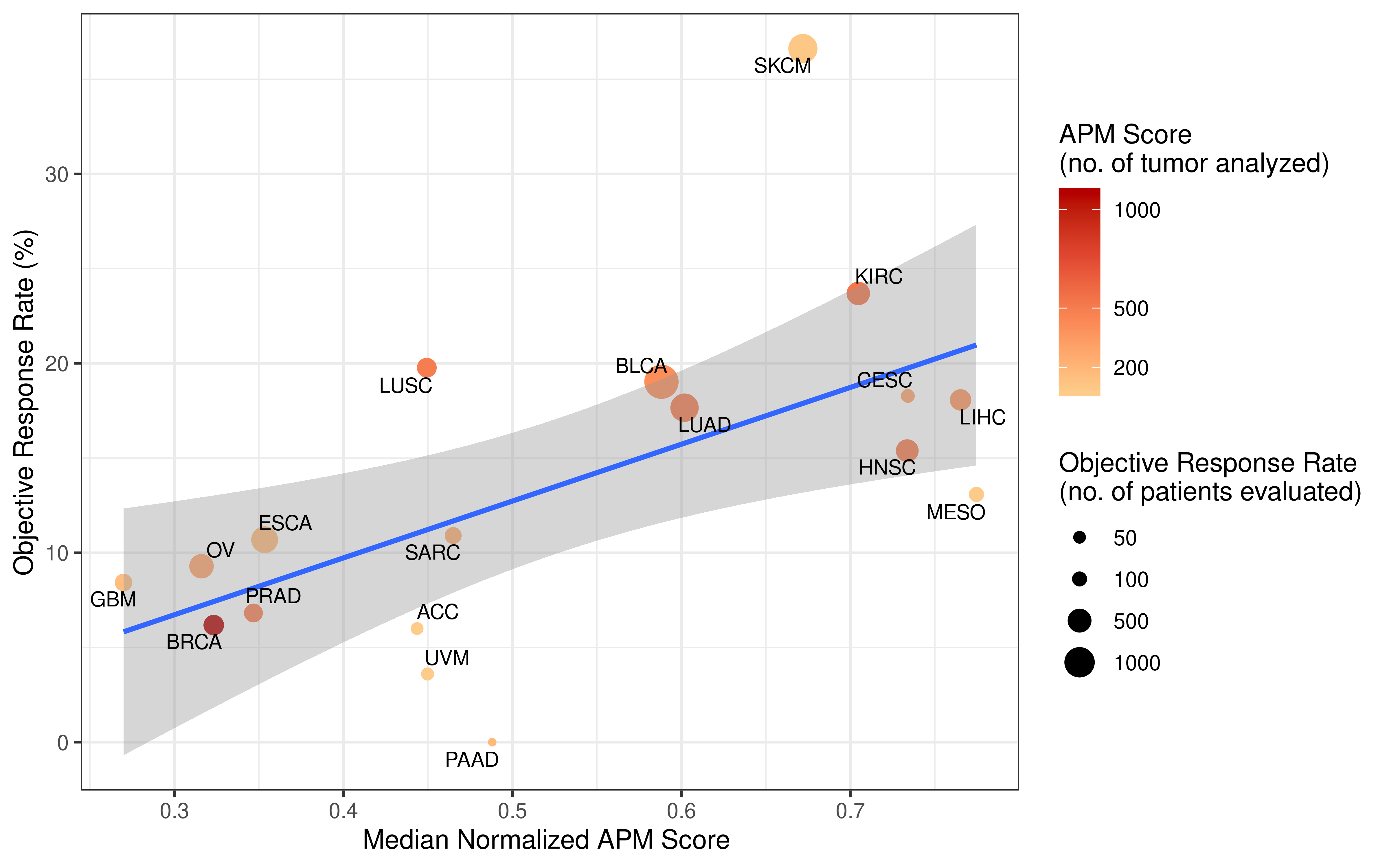
Significant correlation is observed.
lm(ORR ~ APS, filter(tcga_orr, !is.na(ORR))) %>% summary()
#>
#> Call:
#> lm(formula = ORR ~ APS, data = filter(tcga_orr, !is.na(ORR)))
#>
#> Residuals:
#>    Min     1Q Median     3Q    Max
#> -12.37  -3.92  -1.01   2.54  18.73
#>
#> Coefficients:
#>             Estimate Std. Error t value Pr(>|t|)
#> (Intercept)    -2.27       5.54   -0.41   0.6870
#> APS            30.01      10.03    2.99   0.0086 **
#> ---
#> Signif. codes:  0 '***' 0.001 '**' 0.01 '*' 0.05 '.' 0.1 ' ' 1
#>
#> Residual standard error: 7.1 on 16 degrees of freedom
#> Multiple R-squared:  0.359,  Adjusted R-squared:  0.319
#> F-statistic: 8.96 on 1 and 16 DF,  p-value: 0.00861
R and R square can be given as:
TMB
ggplot(filter(tcga_orr, !is.na(ORR)), aes(x = TMB, y = ORR)) +
  geom_point(aes(color = Patients_TMB, size = Patients_ORR)) +
  geom_smooth(method = "lm", se = T) +
  geom_text_repel(aes(label = Project), size = 3) +
  labs(
    x = "Median No. of Coding Somatic Mutation per MB", y = "Objective Response Rate (%)",
    size = "Objective Response Rate\n(no. of patients evaluated)",
    color = "Tumor Mutational Burden\n(no. of tumor analyzed)"
  ) +
  scale_x_continuous(
    trans = log_trans(),
    breaks = c(2, 10, 20, 30, 40, 50),
    labels = c(2, 10, 20, 30, 40, 50)
  ) +
  scale_size_continuous(breaks = c(50, 100, 500, 1000)) +
  scale_color_gradientn(
    colours = RColorBrewer::brewer.pal(5, name = "OrRd")[-1],
    breaks = c(100, 1000, 5000, 10000)
  ) +
  theme_bw() +
  guides(
    color = guide_colorbar(order = 1)
  )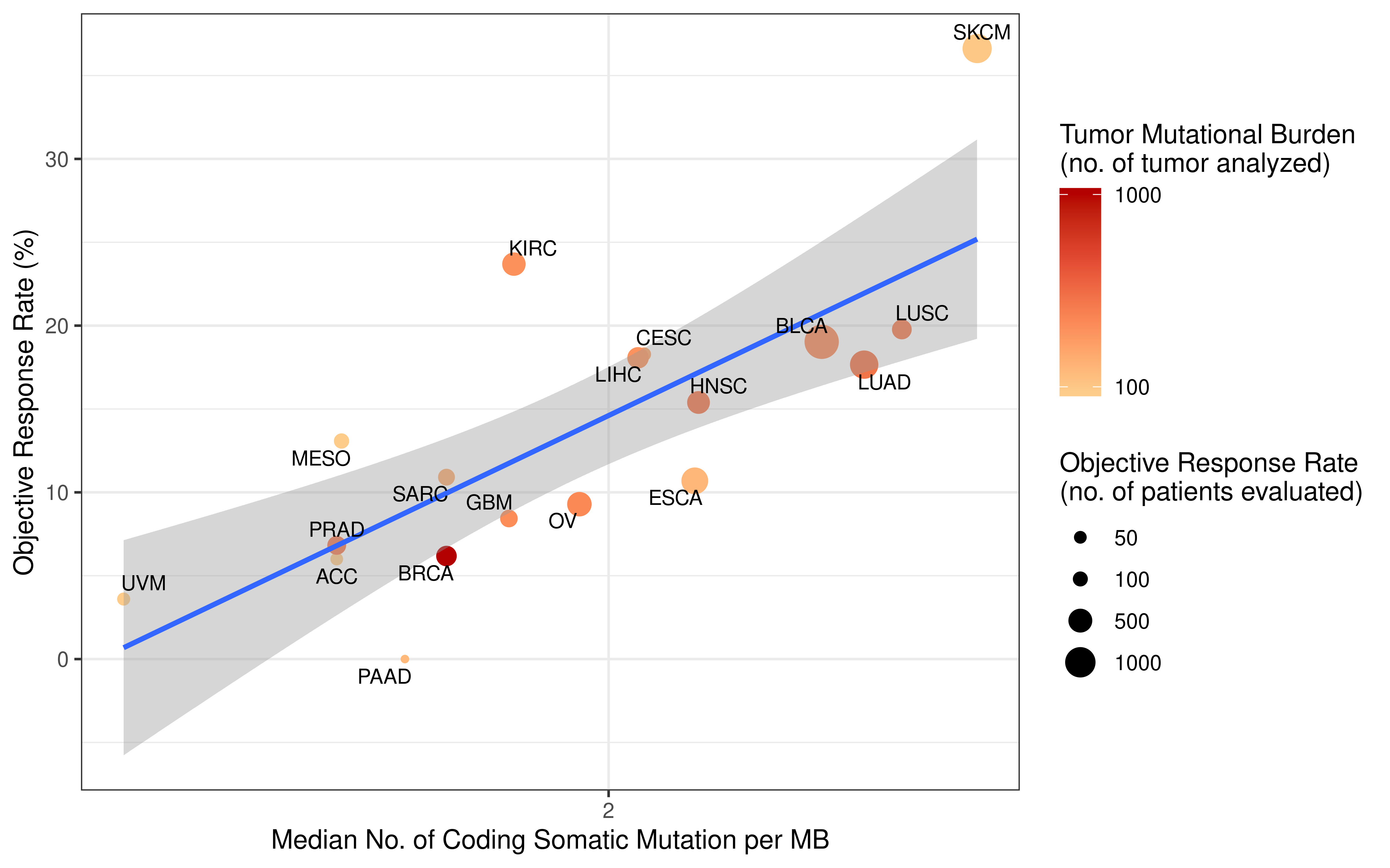
Significant correlation is observed.
lm(ORR ~ TMB, filter(tcga_orr, !is.na(ORR))) %>% summary()
#>
#> Call:
#> lm(formula = ORR ~ TMB, data = filter(tcga_orr, !is.na(ORR)))
#>
#> Residuals:
#>    Min     1Q Median     3Q    Max
#>  -8.69  -3.14  -1.44   4.19  13.51
#>
#> Coefficients:
#>             Estimate Std. Error t value Pr(>|t|)
#> (Intercept)    5.794      1.952    2.97   0.0091 **
#> TMB            3.147      0.602    5.23  8.3e-05 ***
#> ---
#> Signif. codes:  0 '***' 0.001 '**' 0.01 '*' 0.05 '.' 0.1 ' ' 1
#>
#> Residual standard error: 5.4 on 16 degrees of freedom
#> Multiple R-squared:  0.631,  Adjusted R-squared:  0.608
#> F-statistic: 27.3 on 1 and 16 DF,  p-value: 8.28e-05
R and R square can be given as:
TIGS
ggplot(filter(tcga_orr, !is.na(ORR)), aes(x = TIGS, y = ORR)) +
  geom_point(aes(size = Patients_ORR)) +
  geom_smooth(method = "lm", se = T) +
  geom_text_repel(aes(label = Project), size = 3) +
  labs(
    x = "Tumor Immunogenicity Score ", y = "Objective Response Rate (%)",
    size = "Objective Response Rate\n(no. of patients evaluated)"
  ) +
  scale_size_continuous(breaks = c(50, 100, 500, 1000)) +
  theme_bw()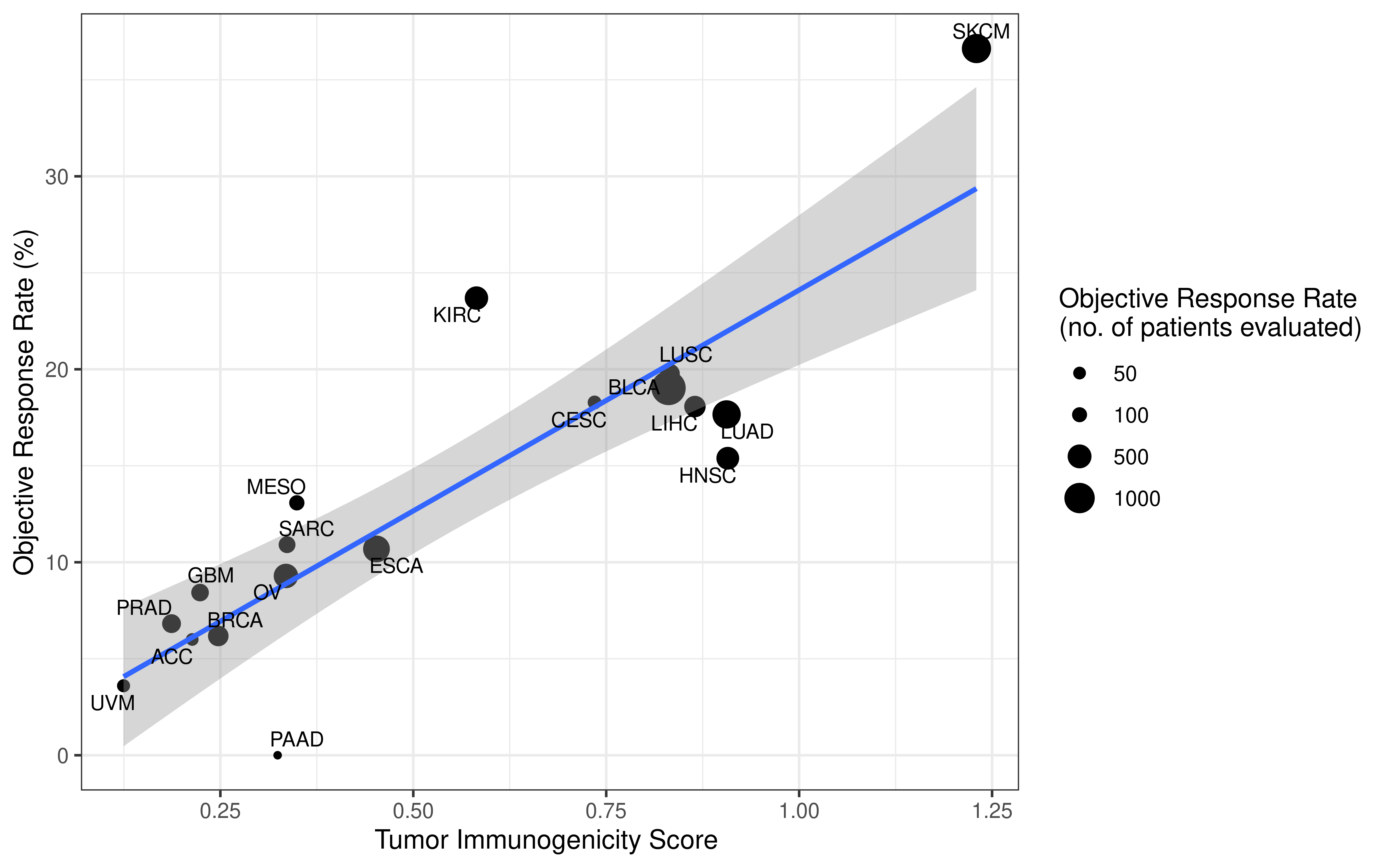
Significant correlation is observed.
lm(ORR ~ TIGS, filter(tcga_orr, !is.na(ORR))) %>% summary()
#>
#> Call:
#> lm(formula = ORR ~ TIGS, data = filter(tcga_orr, !is.na(ORR)))
#>
#> Residuals:
#>    Min     1Q Median     3Q    Max
#> -8.639 -1.122 -0.288  1.826  9.154
#>
#> Coefficients:
#>             Estimate Std. Error t value Pr(>|t|)
#> (Intercept)     1.22       2.04    0.60     0.56
#> TIGS           22.89       3.26    7.02  2.9e-06 ***
#> ---
#> Signif. codes:  0 '***' 0.001 '**' 0.01 '*' 0.05 '.' 0.1 ' ' 1
#>
#> Residual standard error: 4.4 on 16 degrees of freedom
#> Multiple R-squared:  0.755,  Adjusted R-squared:  0.74
#> F-statistic: 49.3 on 1 and 16 DF,  p-value: 2.89e-06
R and R square can be given as:
# R
filter(tcga_orr, !is.na(ORR)) %>%
  summarise(r = cor(ORR, TIGS)) %>%
  pull(r)
#> [1] 0.87
# R square
lm(ORR ~ TIGS, filter(tcga_orr, !is.na(ORR))) %>%
  summary() %>%
  .$r.squared
#> [1] 0.75
These data are consistent with our previous results and even better, which may be caused by fewer included tumor types.
Predict ORR for other tumor types
Using constructed linear formula, we can predict ORR of tumor types which (median) TIGS available.
sm_data <- read_csv("../data/summary_data_new_20190411.csv", col_types = cols())
sm_data$TIGS <- sm_data$Pool_APM * log(sm_data$Pool_TMB + 1)

fit <- lm(Pool_ORR ~ TIGS, filter(sm_data, !is.na(Pool_ORR)))
fit
#>
#> Call:
#> lm(formula = Pool_ORR ~ TIGS, data = filter(sm_data, !is.na(Pool_ORR)))
#>
#> Coefficients:
#> (Intercept)         TIGS
#>       -2.66        21.39
For example , we can predict ORR for uterine corpus endometrial carcinoma (UCEC) on the basis of median TIGS of 0.7.